








Enter the system cost, yearly output, self-use share, retail rate and export rate. If the export rate changes in a later year, also enter the year and the new rate to use two rates. Degradation, upkeep and the analysis period are optional.
Table of Contents
-
What you can do on this page
-
What is this calculation used for?
-
How to Use
-
Formula
-
Symbols and terms
-
Good to know before you start
-
How to calculate it in Excel
-
How to calculate it in Google Sheets
-
How to calculate it in Python
-
How to write it in LaTeX and other math languages (copy and paste)
-
How to have ChatGPT do the calculation
-
DataChef Features
-
Related Features
-
NumberChef Calculators List
What you can do on this page
- Enter the installed cost, yearly output (kWh), self-use share, retail rate and export rate, and you get the first-year benefit (bill savings from self-use + export credits − upkeep) and the simple payback period on the spot
- It also finds the break-even year (the first year the running total of benefits reaches the cost), allowing for panel degradation (0.5% a year by default) and an export rate that changes in a later year, plus the total benefit over the analysis period (20 years by default) and how it compares with the cost
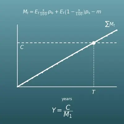
- A year-by-year table (output, self-use, export, benefit, running total) and a chart of the running total show at a glance when it crosses the cost line
- All rates are inputs, so you can use the rates from your own utility plan and net metering or net billing rules
- A plain-language explanation of the formulas and copy-and-paste formulas for Excel, Google Sheets and Python are all on this page
What is this calculation used for?
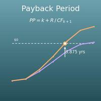
Quotes from different installers differ in cost, system size and estimated yearly production. Putting them all on the same footing, the simple payback (cost ÷ first-year benefit) and the break-even year with degradation, shows differences that the prices alone do not. For example, a quote for $15,000 and 8,000 kWh a year, with a self-use share of 30%, a retail rate of $0.17 and an export rate of $0.12, gives a first-year benefit of about $1,080, a simple payback of about 13.9 years, and a break-even year of year 15.
The key is to use the same formulas and the same rates for every quote. Installer estimates often use different assumptions (rates, self-use share, degradation, rate increases), so it is worth recalculating them yourself on equal terms.
When the retail rate (for example, $0.17/kWh) is higher than the export rate (for example, $0.12/kWh), using 1 kWh yourself is worth more than exporting it. In the example above, raising the self-use share from 30% to 50% increases the first-year benefit from $1,080 to $1,160 (8000 × 0.5 × 0.17 + 8000 × 0.5 × 0.12).
Running the dishwasher or laundry in the middle of the day, charging an electric car at noon, or adding a battery all raise self-use. You can estimate their effect just by changing the self-use share.
Some export rules lock in a rate for a set number of years, after which it changes, and utilities can change their rules for new customers. For example, if the export rate drops from $0.12 to $0.05 in year 11, the benefit in year 11 in the example above falls from about $1,027 to about $654, and the break-even year moves from year 15 to year 17.
Entering the change year and the new rate lets you judge by the running total, including the years after the drop. The longer the period after the drop, the more a high self-use share pays off.
A solar system is not finished once it is installed. There are occasional checkups, and a string inverter often needs replacing after about 10 to 15 years. For example, setting aside $1,500 to $2,500 for an inverter over 15 years plus checkups comes to roughly $150 a year. With $150 of upkeep, the first-year benefit in the example drops to $930 and the break-even year moves from year 15 to year 17.
Leaving upkeep at 0 makes the payback look shorter, so entering the yearly cost over the equipment's life gives a more realistic estimate.
Panel warranties differ by maker (for example, at least 80% after 25 years, or at least 87% after 30 years), and the degradation rates they imply range from about 0.5% to 0.9% a year. In the example above, lowering degradation from 0.5% to 0.3% raises the 20-year total from about $20,604 to about $20,995, about $391 more.
Over a long period, small differences in the rate add up, so this is a way to see in numbers why the warranty terms matter when you choose panels.
Putting solar on an apartment building, a store or a warehouse works the same way: find each year's benefit and the running total from the cost, yearly output, self-use share, retail rate, export rate and upkeep. Businesses often use most of their power in the daytime, so the self-use share tends to be high. On the other hand, tax treatment (such as depreciation and tax credits), commercial rate structures (such as demand charges) and interest need to be considered separately.
This calculation shows only the economics of the equipment itself, without taxes, interest or incentives. For a business decision, talk with a tax professional and the installer, and make the investment decision yourself.
Formula
Symbols and terms
Symbols
| \(C\) | C | The system cost ($), the total price of the solar system including installation. From the first letter of "cost". |
| \(E\) | E | The first-year output (kWh). From the first letter of "energy". |
| \(t\) | t | The year number (1, 2, 3, …). From the first letter of "time". Year 1 is \(t = 1\). |
| \(d\) | d | The degradation rate (%/yr), how much the output drops each year as the panels age. From the first letter of "degradation". |
| \(E_t\) | E sub t | The output in year \(t\) (kWh). The small \(t\) shows which year it is. |
| \(s\) | s | The self-use share (%), the share of the output your home uses directly. From the first letter of "self-consumption". |
| \(p_{\mathrm{b}}\) | p sub b | The retail rate ($/kWh), what you pay the utility for 1 kWh. From "price" and "buy". |
| \(p_{\mathrm{s}}\) | p sub s | The export rate ($/kWh), the credit for 1 kWh sent to the grid. From "price" and "sell". |
| \(m\) | m | The yearly upkeep ($/yr), costs you pay every year such as checkups or money set aside to replace the inverter. From the first letter of "maintenance". |
| \(A_t\) | A sub t | The bill savings from self-use in year \(t\) ($), the cost of the electricity you did not have to buy. |
| \(B_t\) | B sub t | The export credits in year \(t\) ($). It is the item after \(A_t\), so it uses the next letter, \(B\). |
| \(M_t\) | M sub t | The benefit in year \(t\) ($), found as \(A_t + B_t - m\). From the first letter of "merit". |
| \(Y\) | Y | The simple payback (years), the cost divided by the first-year benefit. From the first letter of "year". |
| \(T\) | capital T | The break-even year, the first year the running total reaches the cost. It is the year number \(t\) in capital form, marking one special year. |
| \(\sum\) | sigma | The symbol for "add them all up", the Greek letter S (for sum). \(\sum_{t=1}^{T} M_t\) means "add everything from \(M_1\) to \(M_T\)". |
Terms
| self-use | Using solar power in your own home as it is made, instead of sending it to the grid. You do not have to buy that electricity, so you save the retail rate for each kWh. It is also called self-consumption. |
| self-use share | The share (%) of the output your home uses directly. It is higher when you use more electricity in the daytime; about 30% is typical for a home that is empty during the day. |
| net metering | A billing rule in which the kWh you send to the grid are credited at the same rate you pay, so they cancel out kWh you buy later. The rules differ by state and utility, and some places have changed or ended it. |
| net billing | A billing rule in which you pay the retail rate for the kWh you buy but are credited a lower export rate for the kWh you send to the grid. With net billing, self-use is worth more than export. |
| share kept each year | The share of last year's output that remains. With degradation of 0.5%, it is \(1 - 0.5 \div 100 = 0.995\); multiplying by it once for each year passed gives the output in year \(t\). |
| analysis period | How many years of benefits to add up. 20 to 25 years is common, in line with panel warranties and equipment life (20 years by default on this page). |
| degradation rate | How fast panel output drops as the years go by (%/yr). Studies of real systems often use about 0.5%. Working back from a warranty (for example, at least 80% after 25 years) gives about 0.9%, which usually leaves extra margin. |
| yearly benefit | How much better off you are in a year because of the solar system - the bill savings plus the export credits, minus the yearly upkeep. |
| simple payback | A payback estimate found by dividing the cost by the first-year benefit. It assumes the same benefit every year, so it ignores degradation and rate changes. |
| running total | The total you get by adding year after year from year 1. The running total of benefits is the sum of the yearly benefits from year 1 to that year. It is also called the cumulative total. |
| break-even year | The first year the running total of yearly benefits reaches the system cost. It is a payback that reflects degradation and rate changes. |
| prorate | To split something in proportion. On this page, the decimal part of the payback comes from the ratio of the amount still missing to that year's benefit, which shows where within the break-even year the total is reached. |
| inverter | The device that changes the DC power from the panels into AC power for the home. A string inverter often needs replacing after about 10 to 15 years, so its cost is sometimes planned for as yearly upkeep. |
| performance warranty | A maker's promise that a panel will still produce at least a set percentage of its rated power after a set number of years. It is a basis for choosing a degradation rate. |
| kWh (kilowatt-hour) | The unit for an amount of electricity. Using 1 kW of power for 1 hour is 1 kWh. Both your electric bill and your export credits are based on kWh. |
| power (exponent) | Multiplying the same number by itself several times. \(0.995^{14}\) is 0.995 multiplied 14 times; the small raised number (the exponent) is how many times. |
Good to know before you start
Here is what helps you use the calculation on this page with real understanding, not just by pressing the button.
If you get stuck, going back over these topics is the quickest way forward.
| Percents (Grades 6–7) |
|
| Multiplying and dividing decimals (Grades 5–6) |
|
| Exponents (Grades 6–8) |
|
| Sums of sequences (high school algebra) |
|
| Power and energy (middle school physical science) |
|
How to calculate it in Excel
| First-year output (kWh) | 8000 |
| Degradation rate (%/yr) | 0.5 |
| Year number t | 15 |
| Output in year t (kWh) | =B1*(1-B2/100)^(B3-1) |
| First-year output (kWh) | 8000 |
| Self-use share (%) | 30 |
| Retail rate ($/kWh) | 0.17 |
| Export rate ($/kWh) | 0.12 |
| Yearly upkeep ($/yr) | 0 |
| Bill savings from self-use ($) | =B1*B2/100*B3 |
| Export credits ($) | =B1*(1-B2/100)*B4 |
| Yearly benefit ($) | =B6+B7-B5 |
| System cost ($) | 15000 |
| First-year benefit ($) | 1080 |
| Simple payback (years) | =B1/B2 |
| System cost ($) | 15000 |
| First-year output (kWh) | 8000 |
| Self-use share (%) | 30 |
| Retail rate ($/kWh) | 0.17 |
| Export rate ($/kWh) | 0.12 |
| Degradation rate (%/yr) | 0.5 |
| Yearly upkeep ($/yr) | 0 |
| Running total through year 1 ($) | =B2*(1-B6/100)^0*(B3/100*B4+(1-B3/100)*B5)-B7 |
| Running total through year 2 ($) | =B8+B2*(1-B6/100)^1*(B3/100*B4+(1-B3/100)*B5)-B7 |
| Running total through year 3 ($) | =B9+B2*(1-B6/100)^2*(B3/100*B4+(1-B3/100)*B5)-B7 |
| Running total through year 4 ($) | =B10+B2*(1-B6/100)^3*(B3/100*B4+(1-B3/100)*B5)-B7 |
| Running total through year 5 ($) | =B11+B2*(1-B6/100)^4*(B3/100*B4+(1-B3/100)*B5)-B7 |
| Running total through year 6 ($) | =B12+B2*(1-B6/100)^5*(B3/100*B4+(1-B3/100)*B5)-B7 |
| Running total through year 7 ($) | =B13+B2*(1-B6/100)^6*(B3/100*B4+(1-B3/100)*B5)-B7 |
| Running total through year 8 ($) | =B14+B2*(1-B6/100)^7*(B3/100*B4+(1-B3/100)*B5)-B7 |
| Running total through year 9 ($) | =B15+B2*(1-B6/100)^8*(B3/100*B4+(1-B3/100)*B5)-B7 |
| Running total through year 10 ($) | =B16+B2*(1-B6/100)^9*(B3/100*B4+(1-B3/100)*B5)-B7 |
| Running total through year 11 ($) | =B17+B2*(1-B6/100)^10*(B3/100*B4+(1-B3/100)*B5)-B7 |
| Running total through year 12 ($) | =B18+B2*(1-B6/100)^11*(B3/100*B4+(1-B3/100)*B5)-B7 |
| Running total through year 13 ($) | =B19+B2*(1-B6/100)^12*(B3/100*B4+(1-B3/100)*B5)-B7 |
| Running total through year 14 ($) | =B20+B2*(1-B6/100)^13*(B3/100*B4+(1-B3/100)*B5)-B7 |
| Running total through year 15 ($) | =B21+B2*(1-B6/100)^14*(B3/100*B4+(1-B3/100)*B5)-B7 |
| Running total through year 16 ($) | =B22+B2*(1-B6/100)^15*(B3/100*B4+(1-B3/100)*B5)-B7 |
| Running total through year 17 ($) | =B23+B2*(1-B6/100)^16*(B3/100*B4+(1-B3/100)*B5)-B7 |
| Running total through year 18 ($) | =B24+B2*(1-B6/100)^17*(B3/100*B4+(1-B3/100)*B5)-B7 |
| Running total through year 19 ($) | =B25+B2*(1-B6/100)^18*(B3/100*B4+(1-B3/100)*B5)-B7 |
| Running total through year 20 ($) | =B26+B2*(1-B6/100)^19*(B3/100*B4+(1-B3/100)*B5)-B7 |
| Break-even year | =COUNTIF(B8:B27,"<"&B1)+1 |
| 20-year running total − system cost ($) | =B27-B1 |
The first table is the 8,000 kWh, 0.5% example, and B4 shows the output in year 15, about 7457.8 (kWh). The second table finds the first-year benefit: B6 shows 408 (bill savings), B7 shows 672 (export credits) and B8 shows 1080 (benefit). The third table divides the $15,000 cost by that $1,080, and B3 shows about 13.89 (years).
The fourth table adds up 20 years of benefits one year at a time. Each year's formula adds "first-year output × share kept to the power of (year − 1) × (self-use share ÷ 100 × retail rate + share exported × export rate) − upkeep" to the running total of the year before. The running total in year 15 (B22) is about 15645, the first to pass the cost, so B28 shows 15 (the break-even year) and B29 (20-year running total − cost) shows about 5604 ($). If B28 shows 21, the total does not reach the cost within 20 years. If your export rate changes in a later year, change B5 in the formulas from that year on to point to a cell with the new rate.
How to calculate it in Google Sheets
| First-year output (kWh) | 8000 |
| Degradation rate (%/yr) | 0.5 |
| Year number t | 15 |
| Output in year t (kWh) | =B1*(1-B2/100)^(B3-1) |
| First-year output (kWh) | 8000 |
| Self-use share (%) | 30 |
| Retail rate ($/kWh) | 0.17 |
| Export rate ($/kWh) | 0.12 |
| Yearly upkeep ($/yr) | 0 |
| Bill savings from self-use ($) | =B1*B2/100*B3 |
| Export credits ($) | =B1*(1-B2/100)*B4 |
| Yearly benefit ($) | =B6+B7-B5 |
| System cost ($) | 15000 |
| First-year benefit ($) | 1080 |
| Simple payback (years) | =B1/B2 |
| System cost ($) | 15000 |
| First-year output (kWh) | 8000 |
| Self-use share (%) | 30 |
| Retail rate ($/kWh) | 0.17 |
| Export rate ($/kWh) | 0.12 |
| Degradation rate (%/yr) | 0.5 |
| Yearly upkeep ($/yr) | 0 |
| Running total through year 1 ($) | =B2*(1-B6/100)^0*(B3/100*B4+(1-B3/100)*B5)-B7 |
| Running total through year 2 ($) | =B8+B2*(1-B6/100)^1*(B3/100*B4+(1-B3/100)*B5)-B7 |
| Running total through year 3 ($) | =B9+B2*(1-B6/100)^2*(B3/100*B4+(1-B3/100)*B5)-B7 |
| Running total through year 4 ($) | =B10+B2*(1-B6/100)^3*(B3/100*B4+(1-B3/100)*B5)-B7 |
| Running total through year 5 ($) | =B11+B2*(1-B6/100)^4*(B3/100*B4+(1-B3/100)*B5)-B7 |
| Running total through year 6 ($) | =B12+B2*(1-B6/100)^5*(B3/100*B4+(1-B3/100)*B5)-B7 |
| Running total through year 7 ($) | =B13+B2*(1-B6/100)^6*(B3/100*B4+(1-B3/100)*B5)-B7 |
| Running total through year 8 ($) | =B14+B2*(1-B6/100)^7*(B3/100*B4+(1-B3/100)*B5)-B7 |
| Running total through year 9 ($) | =B15+B2*(1-B6/100)^8*(B3/100*B4+(1-B3/100)*B5)-B7 |
| Running total through year 10 ($) | =B16+B2*(1-B6/100)^9*(B3/100*B4+(1-B3/100)*B5)-B7 |
| Running total through year 11 ($) | =B17+B2*(1-B6/100)^10*(B3/100*B4+(1-B3/100)*B5)-B7 |
| Running total through year 12 ($) | =B18+B2*(1-B6/100)^11*(B3/100*B4+(1-B3/100)*B5)-B7 |
| Running total through year 13 ($) | =B19+B2*(1-B6/100)^12*(B3/100*B4+(1-B3/100)*B5)-B7 |
| Running total through year 14 ($) | =B20+B2*(1-B6/100)^13*(B3/100*B4+(1-B3/100)*B5)-B7 |
| Running total through year 15 ($) | =B21+B2*(1-B6/100)^14*(B3/100*B4+(1-B3/100)*B5)-B7 |
| Running total through year 16 ($) | =B22+B2*(1-B6/100)^15*(B3/100*B4+(1-B3/100)*B5)-B7 |
| Running total through year 17 ($) | =B23+B2*(1-B6/100)^16*(B3/100*B4+(1-B3/100)*B5)-B7 |
| Running total through year 18 ($) | =B24+B2*(1-B6/100)^17*(B3/100*B4+(1-B3/100)*B5)-B7 |
| Running total through year 19 ($) | =B25+B2*(1-B6/100)^18*(B3/100*B4+(1-B3/100)*B5)-B7 |
| Running total through year 20 ($) | =B26+B2*(1-B6/100)^19*(B3/100*B4+(1-B3/100)*B5)-B7 |
| Break-even year | =COUNTIF(B8:B27,"<"&B1)+1 |
| 20-year running total − system cost ($) | =B27-B1 |
How to calculate it in Python
cost_usd = 15000              # system cost ($, installed)
energy_kwh = 8000             # first-year output (kWh)
self_rate_percent = 30        # self-use share (%)
price_buy = 0.17              # retail rate ($/kWh)
price_sell = 0.12             # export rate ($/kWh)
sell_change_year = None       # year the export rate changes (e.g. 11; None if it does not change)
price_sell_after = 0.05       # new export rate ($/kWh)
degradation_percent = 0.5     # degradation rate (%/yr)
maintenance_usd = 0           # yearly upkeep ($/yr)
years = 20                    # analysis period (years)

cumulative = 0
payback_year = None
for t in range(1, years + 1):
    # output in year t = first-year output x (1 - degradation/100)^(t-1)
    energy_t = energy_kwh * (1 - degradation_percent / 100) ** (t - 1)
    sell_price_t = price_sell
    if sell_change_year is not None and t >= sell_change_year:
        sell_price_t = price_sell_after
    saving = energy_t * self_rate_percent / 100 * price_buy          # bill savings from self-use
    income = energy_t * (1 - self_rate_percent / 100) * sell_price_t  # export credits
    merit = saving + income - maintenance_usd                        # yearly benefit
    previous = cumulative
    cumulative += merit
    if payback_year is None and cumulative >= cost_usd:
        payback_year = t
        # point within the year (prorated): amount still missing after last year / this year's benefit
        payback_years = (t - 1) + (cost_usd - previous) / merit
    if t == 1:
        print(f"First-year benefit: ${merit:.0f} (bill savings ${saving:.0f} + export credits ${income:.0f} - upkeep ${maintenance_usd})")
        if merit > 0:
            print(f"Simple payback: {cost_usd / merit:.1f} years")
    print(f"Year {t:2d}: output {energy_t:.1f} kWh / benefit ${merit:.0f} / running total ${cumulative:.0f}")

if payback_year is None:
    print(f"The running total does not reach the system cost within {years} years")
else:
    print(f"Break-even year: year {payback_year} (about {payback_years:.1f} years)")
print(f"{years}-year running total - system cost: ${cumulative - cost_usd:.0f}")
How to write it in LaTeX and other math languages (copy and paste)
Eₜ = E × (1 − d ÷ 100)^(t−1)
E_t = E \times \left(1 - \frac{d}{100}\right)^{t-1}
<math xmlns="http://www.w3.org/1998/Math/MathML" display="block">
<mrow>
<msub><mi>E</mi><mi>t</mi></msub>
<mo>=</mo>
<mi>E</mi>
<mo>×</mo>
<msup>
<mrow><mo>(</mo><mn>1</mn><mo>−</mo><mfrac><mi>d</mi><mn>100</mn></mfrac><mo>)</mo></mrow>
<mrow><mi>t</mi><mo>−</mo><mn>1</mn></mrow>
</msup>
</mrow>
</math>
E_t = E * (1 - d/100)^(t-1)
energyYear = energy*(1 - d/100)^(t - 1)
E_t := E*(1 - d/100)^(t - 1);
E_t = E*(1 - d/100)^(t - 1);
E_t = E×(1−d/100)^(t−1)
Aₜ = Eₜ × (s ÷ 100) × p_b
A_t = E_t \times \frac{s}{100} \times p_{\mathrm{b}}
<math xmlns="http://www.w3.org/1998/Math/MathML" display="block">
<mrow>
<msub><mi>A</mi><mi>t</mi></msub>
<mo>=</mo>
<msub><mi>E</mi><mi>t</mi></msub>
<mo>×</mo>
<mfrac><mi>s</mi><mn>100</mn></mfrac>
<mo>×</mo>
<msub><mi>p</mi><mi mathvariant="normal">b</mi></msub>
</mrow>
</math>
A_t = E_t * (s/100) * p_b
savingYear = energyYear*(s/100)*priceBuy
A_t := E_t*(s/100)*p_b;
A_t = E_t*(s/100)*p_b;
A_t = E_t×(s/100)×p_b
Bₜ = Eₜ × (1 − s ÷ 100) × p_s
B_t = E_t \times \left(1 - \frac{s}{100}\right) \times p_{\mathrm{s}}
<math xmlns="http://www.w3.org/1998/Math/MathML" display="block">
<mrow>
<msub><mi>B</mi><mi>t</mi></msub>
<mo>=</mo>
<msub><mi>E</mi><mi>t</mi></msub>
<mo>×</mo>
<mrow><mo>(</mo><mn>1</mn><mo>−</mo><mfrac><mi>s</mi><mn>100</mn></mfrac><mo>)</mo></mrow>
<mo>×</mo>
<msub><mi>p</mi><mi mathvariant="normal">s</mi></msub>
</mrow>
</math>
B_t = E_t * (1 - s/100) * p_s
incomeYear = energyYear*(1 - s/100)*priceSell
B_t := E_t*(1 - s/100)*p_s;
B_t = E_t*(1 - s/100)*p_s;
B_t = E_t×(1−s/100)×p_s
Mₜ = Aₜ + Bₜ − m
M_t = A_t + B_t - m
<math xmlns="http://www.w3.org/1998/Math/MathML" display="block">
<mrow>
<msub><mi>M</mi><mi>t</mi></msub>
<mo>=</mo>
<msub><mi>A</mi><mi>t</mi></msub>
<mo>+</mo>
<msub><mi>B</mi><mi>t</mi></msub>
<mo>−</mo>
<mi>m</mi>
</mrow>
</math>
M_t = A_t + B_t - m
meritYear = savingYear + incomeYear - maintenance
M_t := A_t + B_t - m;
M_t = A_t + B_t - m;
M_t = A_t + B_t − m
Y = C ÷ M₁
Y = \frac{C}{M_1}
<math xmlns="http://www.w3.org/1998/Math/MathML" display="block">
  <mrow>
    <mi>Y</mi>
    <mo>=</mo>
    <mfrac><mi>C</mi><msub><mi>M</mi><mn>1</mn></msub></mfrac>
  </mrow>
</math>
Y = C / M_1
paybackYears = cost/meritFirstYear
Y := cost/M_1;
Y = cost/M_1;
Y = C/M_1
M₁ + M₂ + ⋯ + M_T ≥ C
\sum_{t=1}^{T} M_t \geq C
<math xmlns="http://www.w3.org/1998/Math/MathML" display="block">
<mrow>
<munderover><mo>∑</mo><mrow><mi>t</mi><mo>=</mo><mn>1</mn></mrow><mi>T</mi></munderover>
<msub><mi>M</mi><mi>t</mi></msub>
<mo>≥</mo>
<mi>C</mi>
</mrow>
</math>
sum_(t=1)^T M_t >= C
paybackYear = First[Select[Range[n], Total[Take[meritList, #]] >= cost &]]
T := min(select(k -> add(M[t], t = 1..k) >= cost, [seq(1..n)]));
T = find(cumsum(M) >= cost, 1);
∑_(t=1)^T M_t ≥ C
How to have ChatGPT do the calculation
You are a calculation assistant for solar payback. Do the following calculation by actually running Python code, and base your answer only on the numbers from the execution result (do not answer by mental math or guessing).

The system cost is $15,000, the first-year output is 8,000 kWh, the self-use share is 30%, the retail rate is $0.17/kWh, the export rate is $0.12/kWh, the degradation rate is 0.5% per year, the yearly upkeep is $0 and the analysis period is 20 years.
Find the output in year t as "first-year output × (1 − 0.5 ÷ 100)^(t − 1)", and the yearly benefit as "output × self-use share ÷ 100 × retail rate + output × (1 − self-use share ÷ 100) × export rate − upkeep".
Find each of the following:
1. The first-year bill savings from self-use, export credits and yearly benefit ($)
2. The simple payback (system cost ÷ first-year benefit, to 1 decimal place)
3. The first year in which the running total of the yearly benefits reaches the system cost (which year)
4. The 20-year running total and its difference from the system cost ($)

Show the formulas you used and the numbers from the execution result. Also note that the result is for the conditions given and does not include tax credits, other incentives, taxes or interest.
How to Use
-
1Enter your numbersType the numbers you want to calculate with into the input fields
-
2CalculatePress the "Calculate" button
-
3Check the resultThe result appears on the spot. The same page also explains the idea behind the calculation and the formula
DataChef Features

No technical knowledge required.
Intuitive and user-friendly operation.

Can be used without registering personal information.

Automatic file deletion by clicking "download".

and rapid file conversion.

No attribution required.

No need to contact us for commercial use permission.
Related Features
Solar Panel Output Calculator (Monthly and Annual kWh from System Size, Peak Sun Hours, Direction and Tilt)
Finds the yearly output (kWh) from the system size, your area's solar radiation, direction and tilt, and losses. Use it to find the "Yearly output" for this page
Payback Period Calculator (Simple and Discounted Payback)
Finds how many years it takes to earn back an investment from the upfront cost and the yearly return. It is the general form of this page's payback, and it can also find a payback that allows for a discount rate
Electric Bill Calculator (kWh to Cost and Back)
Finds your electric bill from the kWh used and your rates. Useful for checking the retail rate (what your self-used solar saves) from your bill