




Choose what to calculate and enter the probabilities. The formula below is linked to the input fields, so you can also calculate by editing the numbers in the formula directly.
Table of Contents
-
What you can do on this page
-
What is this calculation used for?
-
How to Use
-
Formulas and figures
-
Symbols and terms
-
Good to know before you start
-
How to calculate it in Excel
-
How to calculate it in Google Sheets
-
How to calculate it in Python
-
How to write it in LaTeX and other math languages (copy and paste)
-
How to have ChatGPT do the calculation
-
DataChef Features
-
Related Features
-
NumberChef Calculators List
What you can do on this page
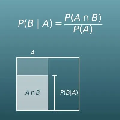
- Enter \(P(A)\) and \(P(A \cap B)\), and you get the conditional probability \(P(B \mid A) = \dfrac{P(A \cap B)}{P(A)}\) on the spot
- In Bayes' theorem mode, you start from the probability of a cause, \(P(A)\), and the probability of a result B with and without that cause, \(P(B \mid A)\) and \(P(B \mid A')\). From these it works backward to "the probability that the cause was A, given that B happened", \(P(A \mid B)\)
- You can follow how \(P(B)\) is built with the law of total probability, in step-by-step formulas with your numbers and in a tree diagram or area model
- Answers are shown both as a fraction in lowest terms (the exact value), such as \(\dfrac{10}{109}\), and as a decimal and a percent
- You can enter a probability as 0.3, 30% or 3/10. A plain-language explanation of the formulas and copy-and-paste formulas for Excel, Google Sheets and Python are included
What is this calculation used for?
"Positive on a 90%-accurate test" sounds like a 90% chance of having the condition. But if you assume, for example, that 1% of all people have it, the probability of really having it after a positive result (the positive predictive value) is only about 9%. The few true positives are buried among the false positives that come from the large group of people who do not have it.
This is the most famous example of Bayes' theorem, and in medicine the basic rule is to read a test result together with the prior probability. (Real probabilities differ from test to test and situation to situation, so these numbers are only an example calculation.)
The classic foundation of spam detection in email apps is a Bayesian filter. From "the probability that this word appears in spam" and "the probability that it appears in normal email", it uses Bayes' theorem to work backward to "the probability that an email containing this word is spam".
Estimating "result to cause" from statistics about "cause (spam) to result (the word appears)" is a textbook application of Bayes' theorem.
A factory has machine X, which makes 60% of the products (2% defective), and machine Y, which makes 40% (5% defective). The probability that a defective product found in inspection came from machine X is, by Bayes' theorem, \(\dfrac{0.6 \times 0.02}{0.6 \times 0.02 + 0.4 \times 0.05} = \dfrac{3}{8}\) (37.5%).
Deciding "which line to inspect first when a defect turns up" can then be based on numbers instead of hunches.
When you draw 2 tickets without putting them back from 10 tickets with 3 winners, the probability that both are winners is \(\dfrac{3}{10} \times \dfrac{2}{9} = \dfrac{1}{15}\). The first result changes the probability of the second (they are not independent), so this is a job for conditional probability and the multiplication rule.
Working out the odds for the rest of the deck from "the cards already showing" in poker, blackjack or other card games is exactly the same calculation.
When setting car insurance premiums, insurers do not look at "the probability of an accident" as one number for everyone. They estimate it as a conditional probability for each condition, such as age, driving record and where you live, and reflect it in different premiums.
The idea of conditional probability, that "the probability changes once you know the condition", supports financial systems such as insurance, loan approval and credit scores.
Formulas and figures
Symbols and terms
Symbols
| \(P(A)\) | P of A | The probability that event A happens. P is the first letter of "probability". |
| \(P(B \mid A)\) | P of B given A | The probability that B happens, given that A is known to have happened (the conditional probability). Some textbooks, for example in Japan, write it as \(P_{A}(B)\), with the condition as a small subscript. |
| \(\mid\) | given | The vertical bar inside \(P(\ \ )\). The event to its right is the condition (what you already know happened), and it is read "given". \(P(B \mid A)\) and \(P(A \mid B)\) mean different things. |
| \(A'\) | A prime (complement) | The event "A does not happen", called the complement of A. Also written \(A^c\) or \(\overline{A}\). It is found with \(P(A') = 1 - P(A)\). |
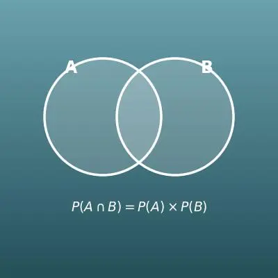
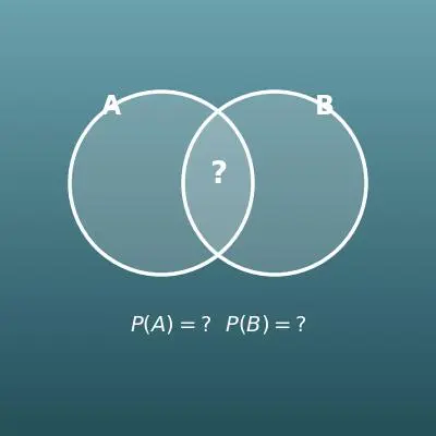
| \(\cap\) | cap (intersection) | The symbol for "and". \(A \cap B\) is the event "both A and B happen". In a Venn diagram it is the part where the two circles overlap. |
| \(P(A \cap B)\) | P of A and B | The probability that both A and B happen (the joint probability). It is the numerator of the conditional probability. It can never be larger than \(P(A)\), because "both happen" is part of A. |
Terms
| event | Something that either happens or does not, such as "rolling an even number" or "testing positive". In probability, such outcomes are called events and are given names like A and B. |
| conditional probability | The probability that an event B happens, under the condition that another event A is known to have happened. It is calculated as \(P(B \mid A) = \dfrac{P(A \cap B)}{P(A)}\). It is "the share of B in a world shrunk from the whole to just A". |
| multiplication rule | The formula \(P(A \cap B) = P(A) \times P(B \mid A)\). It is the conditional probability formula with the denominator cleared, and finds the probability of "first A, and then B too" by multiplying in order. Also called the general multiplication rule. |
| law of total probability | A rule that finds the probability of B by splitting it into "the route through A" and "the route through not A" and adding them. The formula is \(P(B) = P(A)\,P(B \mid A) + P(A')\,P(B \mid A')\). It is used to build the denominator of Bayes' theorem. |
| Bayes' theorem | A rule that works backward from the probability of "cause to result" to the probability of "result to cause". The formula is \(P(A \mid B) = \dfrac{P(A \cap B)}{P(B)}\). It is named after Thomas Bayes, an 18th-century English minister, and it supports modern technology such as spam filters. |
| prior probability | The probability of cause A, \(P(A)\), estimated before you see the result (the data). In the test example, it is "how many people have the condition in the first place". |
| posterior probability | The probability of cause A after it is updated by seeing the result B, \(P(A \mid B)\). Bayes' theorem can be described as a rule that "updates the prior probability to the posterior probability using what you observed". |
| complement | The opposite event, that the event does not happen. The symbol is \(A'\) and its probability is \(1 - P(A)\). In the law of total probability it covers "the route that does not go through A". |
| mutually exclusive | Two events that cannot happen at the same time. "Reaching B through A" and "reaching B through not A" are mutually exclusive, so in the law of total probability you can simply add them. |
| independent | When one result does not change how likely the other is. In terms of conditional probability, A and B are independent when \(P(B \mid A) = P(B)\) (knowing that A happened does not change the probability of B). |
| false positive | A test result that says "positive" even though the person does not really have the condition. Even when the false positive rate is small, if most people do not have the condition, the number of false positives can be larger than the number of true positives. |
| tree diagram | A diagram that lays out the possible cases like the branches of a tree. You write a probability on each branch, and multiplying along a path gives the probability of that route. It is the best diagram for following conditional probability and Bayes' theorem by eye. |
Good to know before you start
Here is what helps you use the calculation on this page with real understanding, not just by pressing the button.
If you get stuck, going back over the topics in this list is the fastest way forward.
| Basic probability (Grade 7) |
|
| Percents and decimals (Grade 6) |
|
| Multiplying and dividing fractions (Grades 5–6) |
|
| Counting outcomes and tree diagrams (Grade 7) |
|
| Sets and Venn diagrams (high school) |
|
How to calculate it in Excel
| Probability of A, P(A) | 0.5 |
| Both A and B, P(A∩B) | 0.2 |
| Conditional probability P(B|A) | =B2/B1 |
| Probability of A, P(A) | 0.5 |
| B given A, P(B|A) | 0.4 |
| Both A and B, P(A∩B) | =B1*B2 |
| Probability of cause A, P(A) | 0.01 |
| B given A, P(B|A) | 0.9 |
| B given not A, P(B|A') | 0.09 |
| Probability of B, P(B) | =B1*B2+(1-B1)*B3 |
| Probability of cause A, P(A) | 0.01 |
| B given A, P(B|A) | 0.9 |
| B given not A, P(B|A') | 0.09 |
| Both A and B, P(A∩B) | =B1*B2 |
| Probability of B, P(B) | =B4+(1-B1)*B3 |
| Cause is A, given B, P(A|B) | =B4/B5 |
In a formula, "B1" and "B2" mean "use the number in that cell", "*" is multiplication and "/" is division.
The first table gives 0.2 ÷ 0.5 = 0.4, and the second gives 0.5 × 0.4 = 0.2.
The third table gives 0.01 × 0.9 + 0.99 × 0.09 = 0.0981, adding up the probability of a positive test route by route.
In the fourth table, B4 is 0.009 and B5 is 0.0981, and the last cell, B6, is 0.009 ÷ 0.0981 ≈ 0.0917 (about 9.2%).
How to calculate it in Google Sheets
| Probability of A, P(A) | 0.5 |
| Both A and B, P(A∩B) | 0.2 |
| Conditional probability P(B|A) | =B2/B1 |
| Probability of A, P(A) | 0.5 |
| B given A, P(B|A) | 0.4 |
| Both A and B, P(A∩B) | =B1*B2 |
| Probability of cause A, P(A) | 0.01 |
| B given A, P(B|A) | 0.9 |
| B given not A, P(B|A') | 0.09 |
| Probability of B, P(B) | =B1*B2+(1-B1)*B3 |
| Probability of cause A, P(A) | 0.01 |
| B given A, P(B|A) | 0.9 |
| B given not A, P(B|A') | 0.09 |
| Both A and B, P(A∩B) | =B1*B2 |
| Probability of B, P(B) | =B4+(1-B1)*B3 |
| Cause is A, given B, P(A|B) | =B4/B5 |
Just replace the input numbers with your own probabilities.
How to calculate it in Python
from fractions import Fraction

# ===== Conditional probability P(B|A) = P(A∩B) ÷ P(A) =====
p_a = Fraction(1, 2)          # P(A): probability of the given event A
p_a_and_b = Fraction(1, 3)    # P(A∩B): probability that both happen
p_b_given_a = p_a_and_b / p_a
print(f"Conditional probability P(B|A): {p_b_given_a} = {float(p_b_given_a):.4f}")

# ===== Bayes' theorem (the denominator is built with the law of total probability) =====
prior = Fraction(1, 100)             # P(A): probability of cause A (prior probability)
p_b_given_a2 = Fraction(90, 100)     # P(B|A): probability of B given A
p_b_given_not_a = Fraction(9, 100)   # P(B|A'): probability of B given not A

p_joint = prior * p_b_given_a2                    # P(A∩B)
p_b = p_joint + (1 - prior) * p_b_given_not_a     # P(B) (law of total probability)
posterior = p_joint / p_b                         # P(A|B) (posterior probability)
print(f"Probability of B, P(B): {p_b} = {float(p_b):.4f}")
print(f"Probability the cause is A, P(A|B): {posterior} = {float(posterior):.4f}")
How to write it in LaTeX and other math languages (copy and paste)
P(B|A) = P(A∩B) / P(A)
P(B \mid A) = \dfrac{P(A \cap B)}{P(A)}
<math xmlns="http://www.w3.org/1998/Math/MathML" display="block">
<mrow>
<mi>P</mi><mo>(</mo><mi>B</mi><mo>∣</mo><mi>A</mi><mo>)</mo>
<mo>=</mo>
<mfrac>
<mrow><mi>P</mi><mo>(</mo><mi>A</mi><mo>∩</mo><mi>B</mi><mo>)</mo></mrow>
<mrow><mi>P</mi><mo>(</mo><mi>A</mi><mo>)</mo></mrow>
</mfrac>
</mrow>
</math>
P(B | A) = P(A nn B) / P(A)
pAandB/pA
pBgivenA := pAandB/pA;
p_b_given_a = p_a_and_b/p_a;
P(B|A) = P(A∩B)/P(A)
P(A∩B) = P(A) × P(B|A)
P(A \cap B) = P(A) \times P(B \mid A)
<math xmlns="http://www.w3.org/1998/Math/MathML" display="block">
<mrow>
<mi>P</mi><mo>(</mo><mi>A</mi><mo>∩</mo><mi>B</mi><mo>)</mo>
<mo>=</mo>
<mi>P</mi><mo>(</mo><mi>A</mi><mo>)</mo>
<mo>×</mo>
<mi>P</mi><mo>(</mo><mi>B</mi><mo>∣</mo><mi>A</mi><mo>)</mo>
</mrow>
</math>
P(A nn B) = P(A) xx P(B | A)
pA*pBgivenA
pAandB := pA*pBgivenA;
p_a_and_b = p_a*p_b_given_a;
P(A∩B) = P(A) × P(B|A)
P(B) = P(A) × P(B|A) + P(A′) × P(B|A′)
P(B) = P(A)\,P(B \mid A) + P(A')\,P(B \mid A')
<math xmlns="http://www.w3.org/1998/Math/MathML" display="block">
<mrow>
<mi>P</mi><mo>(</mo><mi>B</mi><mo>)</mo>
<mo>=</mo>
<mi>P</mi><mo>(</mo><mi>A</mi><mo>)</mo>
<mi>P</mi><mo>(</mo><mi>B</mi><mo>∣</mo><mi>A</mi><mo>)</mo>
<mo>+</mo>
<mi>P</mi><mo>(</mo>
<msup><mi>A</mi><mo>′</mo></msup>
<mo>)</mo>
<mi>P</mi><mo>(</mo><mi>B</mi><mo>∣</mo>
<msup><mi>A</mi><mo>′</mo></msup>
<mo>)</mo>
</mrow>
</math>
P(B) = P(A) xx P(B | A) + P(A') xx P(B | A')
pA*pBgivenA + (1 - pA)*pBgivenNotA
pB := pA*pBgivenA + (1 - pA)*pBgivenNotA;
p_b = p_a*p_b_given_a + (1 - p_a)*p_b_given_not_a;
P(B) = P(A)P(B|A) + P(A′)P(B|A′)
P(A|B) = P(A∩B) / P(B)
P(A \mid B) = \dfrac{P(A \cap B)}{P(B)} = \dfrac{P(A)\,P(B \mid A)}{P(A)\,P(B \mid A) + P(A')\,P(B \mid A')}
<math xmlns="http://www.w3.org/1998/Math/MathML" display="block">
<mrow>
<mi>P</mi><mo>(</mo><mi>A</mi><mo>∣</mo><mi>B</mi><mo>)</mo>
<mo>=</mo>
<mfrac>
<mrow><mi>P</mi><mo>(</mo><mi>A</mi><mo>∩</mo><mi>B</mi><mo>)</mo></mrow>
<mrow><mi>P</mi><mo>(</mo><mi>B</mi><mo>)</mo></mrow>
</mfrac>
</mrow>
</math>
P(A | B) = P(A nn B) / P(B)
pA*pBgivenA/(pA*pBgivenA + (1 - pA)*pBgivenNotA)
pAgivenB := pAandB/pB;
p_a_given_b = p_a_and_b/p_b;
P(A|B) = P(A∩B)/P(B)
How to have ChatGPT do the calculation
You are a calculation assistant for probability (conditional probability and Bayes' theorem). Do the following calculation by actually running Python code, and base your answer only on the numbers from the execution result (do not answer by mental math or guessing).

The probability of cause A (the prior probability) is 1%. The probability of result B when A happens, P(B|A), is 90%. The probability of B when A does not happen, P(B|A'), is 9%.
Find each of the following:
1. The probability that both A and B happen, P(A∩B)
2. The probability of B, P(B) (using the law of total probability, and also show the breakdown by route)
3. The probability that the cause is A, given that B happened, P(A|B) (Bayes' theorem; show it both as a fraction in lowest terms and as a decimal)

In Python, use the fractions module from the standard library to calculate exactly, and show the formulas you used and the numbers from the execution result in a table.
How to Use
-
1Enter your numbersType the numbers you want to calculate with into the input fields
-
2CalculatePress the "Calculate" button
-
3Check the resultThe result appears on the spot. The same page also explains the idea behind the calculation and the formula
DataChef Features

No technical knowledge required.
Intuitive and user-friendly operation.

Can be used without registering personal information.

Automatic file deletion by clicking "download".

and rapid file conversion.

No attribution required.

No need to contact us for commercial use permission.
Related Features
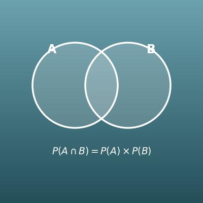
Probability of Two Events (And, Or, Neither)
Finds the probability that both happen, that at least one happens, and more, from two probabilities
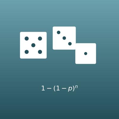
Probability of Repeated Trials (n in a Row, At Least Once)
Finds the probability that something happens n times in a row, or at least once in n tries
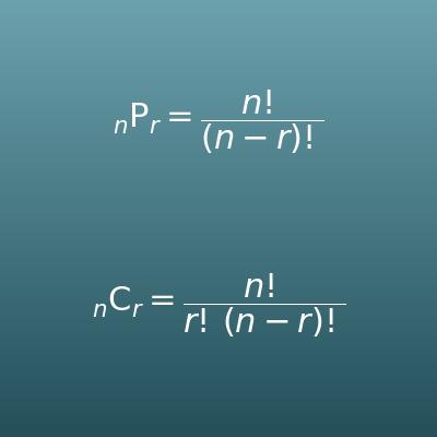
Permutation and Combination Calculator (nPr, nCr)
Counts the number of ways to arrange (permutations) and to choose (combinations)