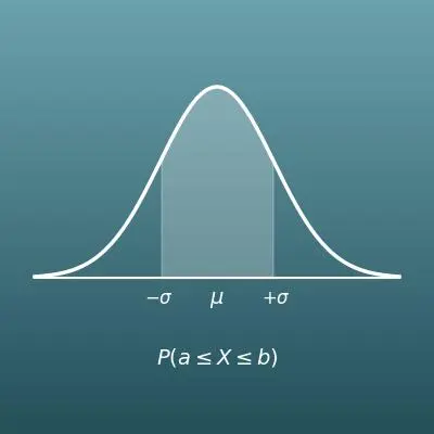

Enter the mean, the standard deviation, and the lower and upper bounds of the range you want. The calculator finds the probability of falling in that range and a confidence interval table.
Table of Contents
-
What you can do on this page
-
What is this calculation used for?
-
How to Use
-
Formula and graph
-
Symbols and terms
-
Good to know before you start
-
How to calculate it in Excel
-
How to calculate it in Google Sheets
-
How to calculate it in Python
-
How to write it in LaTeX and other math languages (copy and paste)
-
How to have ChatGPT do the calculation
-
DataChef Features
-
Related Features
-
NumberChef Calculators List
What you can do on this page
- Enter the mean \(\mu\) and the spread (standard deviation \(\sigma\)), and you get the probability that a value falls in a given range on the spot
- It also finds the probability of being at or above (or at or below) a value, such as "What percent of students scored 80 or higher?"
- A table of the ranges often used in statistics (such as the range that holds 95% of the whole) is shown at the same time
- A plain-language explanation of the normal distribution and copy-and-paste formulas for Excel, Google Sheets and Python are all on this page
What is this calculation used for?
IQ scores are set so that the mean is 100 and one standard deviation is 15 points. In a normal distribution, only about 16% of people are at \(+1\sigma\) or above (an IQ of 115 or more), and only about 2.3% are at \(+2\sigma\) or above (130 or more).
Once you see this link, percentile ranks on standardized tests stop being a mystery. You can read what "a 10-point jump" or "the 90th percentile" really stands for in numbers, not just by feel.
The "reference range" on blood tests and similar lab results is often set as the range that holds the middle 95% of measurements from healthy people (about the mean \(\pm 2\sigma\)).
So for any test item, about 5% of healthy people (1 in 20) fall outside the reference range. On a checkup with many items, it is actually common for a healthy person to be flagged on at least one. Knowing this, you understand that "slightly outside the range" is not automatically a sign that "something is wrong", and you can listen to your doctor's explanation calmly. It is especially useful if test results tend to worry you.
The weights and sizes of products vary in a way that comes close to a normal distribution. For example, if bags labeled 16 oz are filled with an average of 16.2 oz and a standard deviation of 0.1 oz, the bags under 16 oz are those beyond \(-2\sigma\), about 2.3%.
Factories use this calculation to predict the defect rate and to decide where to set the average fill (how much extra to put in) to balance customer complaints against cost.
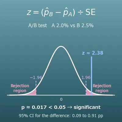
When you compare whether design A or design B gets the higher click-through rate, you use the normal distribution (a confidence interval) to decide whether the difference is just chance or a real difference.
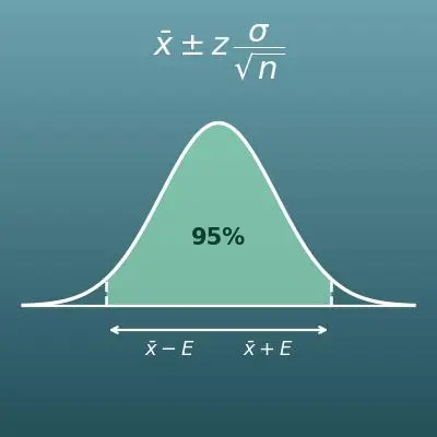
The "0.95" row in the table shown in the result is exactly the "95% confidence interval" used most often in practice. Behind decisions that move large sums of money, such as ad budgets, this calculation is used every day.
Professionals called actuaries estimate the risk of paying out claims as probabilities and set insurance premiums from them.
Single accidents cannot be predicted, but the total over many policyholders comes close to a normal distribution (the central limit theorem), so the total payout can be predicted surprisingly accurately. This math is why we can get large coverage for an affordable premium.
Formula and graph
Symbols and terms
Symbols
| \(\mu\) | mu | The mean. It is where the center of the peak of the distribution sits. A Greek letter that corresponds to the English m. |
| \(\sigma\) | sigma | The standard deviation. It is the size of the spread of the data and sets the width of the peak. The larger it is, the lower and wider the peak. A Greek letter that corresponds to the English s. |
| \(X\) | X (random variable) | A letter for a quantity whose value can change each time you measure it, such as a test score or a height. |
| \(\Phi\) | capital phi | The cumulative distribution function of the standard normal distribution (mean 0, standard deviation 1). It returns the probability of getting that value or less. |
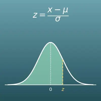
| \(z\) | z (z-score) | A number that tells how many standard deviations a value is from the mean. It is found with \(z = (x - \mu) \div \sigma\). |
| \(e\) | e (Euler's number) | A constant, about 2.71828…, and the base of the natural logarithm. It is a special number at the heart of exponential functions. |
| \(\pi\) | pi | A constant, about 3.14159…, the ratio of a circle's circumference to its diameter. In the normal distribution formula it appears to make the total area under the curve exactly 1. |
Terms
| normal distribution | A distribution spread symmetrically around the mean in a bell shape. It is used as a model for data where values near the mean are the most common and values get rarer the farther they are from the mean, such as heights, test scores and the weights of products. |
| standard deviation | One number that shows how spread out the data is. Two data sets can have the same mean but different spreads. The larger the standard deviation, the lower and wider the peak of the distribution. |
| standardization (z-score) | Rewriting a value as "how many standard deviations it is from the mean" (the \(z\)-score). Any normal distribution, once standardized, can be handled with the single standard normal distribution with mean 0 and standard deviation 1. IQ scores use the same idea: IQ \(= 100 + 15 \times z\). |
| cumulative distribution function | A function that returns the probability of getting that value or less. For the standard normal distribution it is written \(\Phi\) (phi). The probability of a range is "\(\Phi\) up to the upper bound" minus "\(\Phi\) up to the lower bound". |
| probability density function | The formula for the curve of the distribution itself. The height of the curve is not a probability but a probability density. The area between the curve and the horizontal axis over a range is the probability. For the normal distribution, it is a bell-shaped curve. |
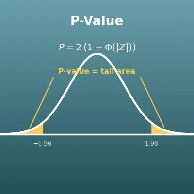
| confidence interval | The table in the result lists, for each percentage, the range centered on the mean that holds that share of the whole distribution (\(\mu \pm z \times \sigma\)) and its multiplier \(z\). Strictly speaking, a "95% confidence interval" in statistics is a range for the true value (such as the population mean) estimated from sample data. But when a normal distribution is assumed, it uses the same \(z\) (1.96 for 95%), so the \(z\) values in this table apply directly. It is often used to find the "margin of error" of surveys and test results. |
| 68–95–99.7 rule | A handy rule of thumb, also called the empirical rule: in a normal distribution, about 68.3% of the data falls within the mean \(\pm 1\sigma\), about 95.4% within \(\pm 2\sigma\), and about 99.7% within \(\pm 3\sigma\). |
| central limit theorem | The mathematical fact that a quantity built up from many small random effects (a sum or an average) gets close to a normal distribution, whatever the original distribution. It is the reason so much real-world data comes close to a normal distribution. |
Good to know before you start
Here is what helps you use the calculation on this page with real understanding, not just by pressing the button.
| The mean (Grade 6) |
|
| Data analysis and standard deviation (high school statistics) |
|
| Reading shares as areas (Grades 6–7) |
|
| Standardization and z-scores (high school statistics / AP Statistics) |
|
How to calculate it in Excel
| Mean μ | 62 |
| Standard dev. σ | 14 |
| Lower bound | 50 |
| Upper bound | 80 |
| Probability between the bounds | =NORM.DIST(B4,B1,B2,TRUE)-NORM.DIST(B3,B1,B2,TRUE) |
| Mean μ | 62 |
| Standard dev. σ | 14 |
| Value (find the share at or above it) | 80 |
| Probability of that value or more | =1-NORM.DIST(B3,B1,B2,TRUE) |
| Mean μ | 62 |
| Standard dev. σ | 14 |
| Point x | 80 |
| Height of the curve at that point | =NORM.DIST(B3,B1,B2,FALSE) |
The probability of a range is "the probability of the upper bound or less" minus "the probability of the lower bound or less".
If you set the last argument to FALSE, you get the height of the curve at that point (the value of the probability density function) instead of a probability.
After pasting, column B holds your inputs and the formula in the last row calculates automatically. The first table shows about 0.70 (about 70%), and the second shows about 0.10 (about 10%, that is, the top 10% or so).
How to calculate it in Google Sheets
| Mean μ | 62 |
| Standard dev. σ | 14 |
| Lower bound | 50 |
| Upper bound | 80 |
| Probability between the bounds | =NORMDIST(B4,B1,B2,TRUE)-NORMDIST(B3,B1,B2,TRUE) |
| Mean μ | 62 |
| Standard dev. σ | 14 |
| Value (find the share at or above it) | 80 |
| Probability of that value or more | =1-NORMDIST(B3,B1,B2,TRUE) |
| Mean μ | 62 |
| Standard dev. σ | 14 |
| Point x | 80 |
| Height of the curve at that point | =NORMDIST(B3,B1,B2,FALSE) |
NORMDIST(x, mean, standard_deviation, TRUE) returns the probability of getting x or less, so the upper bound's value minus the lower bound's value is the probability of the range.
If you set the last argument to FALSE, you get the height of the curve at that point (the probability density) instead of a probability.
How to calculate it in Python
from statistics import NormalDist

mean = 62               # mean
standard_deviation = 14 # standard deviation
lower_bound = 50        # lower bound of the range
upper_bound = 80        # upper bound of the range

distribution = NormalDist(mean, standard_deviation)
p_between = distribution.cdf(upper_bound) - distribution.cdf(lower_bound)

print(f"Probability between {lower_bound} and {upper_bound}: {p_between}")
How to write it in LaTeX and other math languages (copy and paste)
P(a ≤ X ≤ b) = Φ((b − μ)/σ) − Φ((a − μ)/σ)
P(a \le X \le b) = \Phi\!\left(\frac{b-\mu}{\sigma}\right) - \Phi\!\left(\frac{a-\mu}{\sigma}\right)
<math xmlns="http://www.w3.org/1998/Math/MathML" display="block">
<mrow>
<mi>P</mi><mo>(</mo><mi>a</mi><mo>≤</mo><mi>X</mi><mo>≤</mo><mi>b</mi><mo>)</mo>
<mo>=</mo>
<mi>Φ</mi>
<mrow>
<mo>(</mo>
<mfrac><mrow><mi>b</mi><mo>−</mo><mi>μ</mi></mrow><mi>σ</mi></mfrac>
<mo>)</mo>
</mrow>
<mo>−</mo>
<mi>Φ</mi>
<mrow>
<mo>(</mo>
<mfrac><mrow><mi>a</mi><mo>−</mo><mi>μ</mi></mrow><mi>σ</mi></mfrac>
<mo>)</mo>
</mrow>
</mrow>
</math>
P(a <= X <= b) = Phi((b - mu)/sigma) - Phi((a - mu)/sigma)
CDF[NormalDistribution[mu, sigma], b] - CDF[NormalDistribution[mu, sigma], a]
with(Statistics): CDF(RandomVariable(Normal(mu, sigma)), b) - CDF(RandomVariable(Normal(mu, sigma)), a);
p = normcdf(b, mu, sigma) - normcdf(a, mu, sigma);
P(a ≤ X ≤ b) = Φ((b-μ)/σ) - Φ((a-μ)/σ)
f(x) = 1/(σ√(2π)) · e^(−(x − μ)²/(2σ²))
f(x) = \frac{1}{\sigma\sqrt{2\pi}}\, e^{-\frac{(x-\mu)^2}{2\sigma^2}}
<math xmlns="http://www.w3.org/1998/Math/MathML" display="block">
<mrow>
<mi>f</mi><mo>(</mo><mi>x</mi><mo>)</mo>
<mo>=</mo>
<mfrac>
<mn>1</mn>
<mrow><mi>σ</mi><msqrt><mrow><mn>2</mn><mi>π</mi></mrow></msqrt></mrow>
</mfrac>
<msup>
<mi>e</mi>
<mrow>
<mo>−</mo>
<mfrac>
<msup><mrow><mo>(</mo><mi>x</mi><mo>−</mo><mi>μ</mi><mo>)</mo></mrow><mn>2</mn></msup>
<mrow><mn>2</mn><msup><mi>σ</mi><mn>2</mn></msup></mrow>
</mfrac>
</mrow>
</msup>
</mrow>
</math>
f(x) = 1/(sigma sqrt(2 pi)) e^(-(x - mu)^2 / (2 sigma^2))
PDF[NormalDistribution[mu, sigma], x]
with(Statistics): PDF(RandomVariable(Normal(mu, sigma)), x);
y = normpdf(x, mu, sigma);
f(x) = 1/(σ√(2π)) e^(-(x-μ)^2/(2σ^2))
How to have ChatGPT do the calculation
You are a probability calculation assistant. Do the following calculation by actually running Python code, and base your answer only on the numbers from the execution result (do not answer by mental math or guessing).

The scores on a test follow a normal distribution with a mean of 62 points and a standard deviation of 14 points.
Find each of the following:
1. The probability that a score is between 50 and 80 points
2. The probability that a score is 80 points or more (the top what percent)
3. The probability that a score is 50 points or less

Use Python's statistics.NormalDist, and show the code you used and the numbers from the execution result.
How to Use
-
1Enter your numbersType the numbers you want to calculate with into the input fields
-
2CalculatePress the "Calculate" button
-
3Check the resultThe result appears on the spot. The same page also explains the idea behind the calculation and the formula
DataChef Features

No technical knowledge required.
Intuitive and user-friendly operation.

Can be used without registering personal information.

Automatic file deletion by clicking "download".

and rapid file conversion.

No attribution required.

No need to contact us for commercial use permission.
Related Features
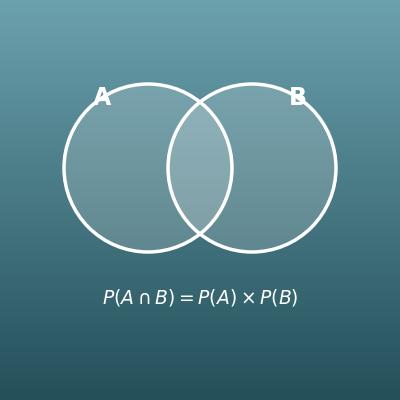
Probability of Two Events (And, Or, Neither)
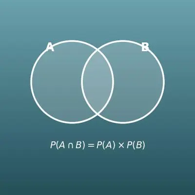
From two probabilities, find the probability that both happen, that at least one happens, and more
Probability of Two Events Solver
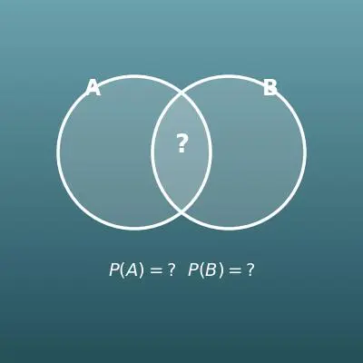
From the two probabilities you know, work out all the other probabilities
Probability of Repeated Trials (n in a Row, At Least Once)
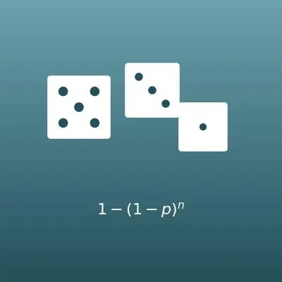
Find the probability that something happens n times in a row, or at least once in n tries
Binomial Distribution Calculator
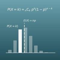
The binomial distribution behind the normal approximation. Find the probability of exactly k successes, cumulative probabilities, and check the np ≥ 5 rule of thumb