


Bookmarks    
nPr and nCr    
Random Number    
SD Calculator    
Sample Size    
Percent Error    
Density    
Molarity    
Molar Mass    
Ohm's Law    
Watts to Amps    
Voltage Drop    
Long Division    
Mixed Numbers    
Rounding    
Nth Root    
Exponents    
Half-Life    
Polar Form    
De Moivre    
3D Distance    
Point to Line    
Cross Product    
Determinant    
Sin Cos Tan    
Triangle Area    
Scale Factor    
Sector Area    
Ellipse Area    
Cube Volume    
Box Volume    
Sphere Volume    
Cone Volume    
Pipe Volume    
Time Duration    
Time Card    
Present Value    
Future Value    
Churn Rate    
A/B Test Calc    
SEO Traffic    
Ideal Weight    
Fat Intake    
Child Height    
Golf Handicap    
Heat Index    
Wind Chill    
Dew Point    
Download Time    
kWh to Cost    
AC Size (BTU)    
Heating Costs    
LED Savings    
Trip Gas Cost    
Tire Size    
Solar Output    
Solar Payback    
Battery Size    
Wall Area    
Gravel Needed    
Mortar Mix    
Slope Grade    
Curtain Size    
Soil Needed    
Sod Needed    
Ramp Length    
Blind Size    
Drain Slope    
Board Feet    
Heat Loss    
Furniture Fit    
Moving Boxes    
Plywood Cuts    
Shelf Sag    
   Add
Probability and random number calculators
Independent Events
Independent Events
Two Events Solver
Two Events Solver
Repeated Trials
Repeated Trials
Bayes' Theorem
Bayes' Theorem
Expected Value
Expected Value
Binomial Distribution
nPr and nCr
nPr and nCr
Circular Permutation
With Repetition
With Repetition
Random Number
Random Number
Averages and statistics calculators
Average Calculator
Average Calculator
Mean Median Mode
Mean Median Mode
SD Calculator
SD Calculator
Quartiles & IQR
Quartiles & IQR
Frequency Table
Frequency Table
Correlation (r)
Correlation (r)
Normal Probability
Normal Probability
Z-Score Calculator
Z-Score Calculator
Confidence Interval
Confidence Interval
Sample Size
Sample Size
Mark & Recapture
Mark & Recapture
P-Value Calculator
P-Value Calculator
Percentage and ratio calculators
Percentage Calc
Percentage Calc
Percent Change
Percent Change
Percent Difference
Percent Difference
Percent Error
Percent Error
Ratio Calculator
Ratio Calculator
Discount Calculator
Discount Calculator
Sales Tax Calculator
Margin Calculator
Margin Calculator
Speed calculators
Speed Calculator
Speed Calculator
Density and concentration calculators
Density
Density
Molarity
Molarity
Molar Mass
Molar Mass
Physics and electricity calculators
Ohm's Law
Ohm's Law
Watts to Amps
Watts to Amps
Resistor Colors
Resistor Colors
Voltage Drop
Voltage Drop
Unit conversion calculators
Weight Converter
Weight Converter
Shoe Size Converter
Shoe Size Converter
Integer and signed number calculators
Long Division
Long Division
LCM Calculator
LCM Calculator
GCF Calculator
GCF Calculator
Integer Calculator
Integer Calculator
Prime Factorization
Prime Factorization
Diophantine Solver
Diophantine Solver
Modulo Calculator
Modulo Calculator
Factor Calculator
Factor Calculator
Roman Numerals
Roman Numerals
Fraction, decimal and rounding calculators
Fraction Calculator
Fraction Calculator
Mixed Numbers
Mixed Numbers
Simplify Fractions
Simplify Fractions
Fraction to Decimal
Fraction to Decimal
Decimal to Fraction
Decimal to Fraction
Rounding
Rounding
Equation and inequality calculators
Linear Equation
Linear Equation
Linear Systems
Linear Systems
Quadratic Formula
Quadratic Formula
Absolute Value
Absolute Value
Quadratic Inequality
Polynomial calculators
Binomial Theorem
Binomial Theorem
Square root and nth root calculators
Simplify Radicals
Simplify Radicals
Nth Root
Nth Root
Exponent and logarithm calculators
Exponents
Exponents
Log Calculator
Log Calculator
Number of Digits
Number of Digits
Scientific Notation
Scientific Notation
Sci. Notation Math
Sci. Notation Math
Half-Life
Half-Life
Complex number calculators
Complex Numbers
Complex Numbers
Polar Form
Polar Form
De Moivre
De Moivre
Function and graph calculators
Slope Calculator
Slope Calculator
Linear Function
Linear Function
Direct & Inverse Variation
y = ax² Calculator
y = ax² Calculator
Distance Formula
Distance Formula
3D Distance
3D Distance
Section Formula
Section Formula
Point to Line
Point to Line
Lat/Long Distance
Lat/Long Distance
Complete the Square
Complete the Square
Circle Equation
Circle Equation
Conic Sections
Conic Sections
Polar Coordinates
Polar Coordinates
Sequence calculators
Arithmetic Sequence
Arithmetic Sequence
Geometric Sequence
Geometric Sequence
Fibonacci Sequence
Fibonacci Sequence
Recurrence Relation
Recurrence Relation
Vector calculators
Vector Calculator
Vector Calculator
Cross Product
Cross Product
Matrix calculators
Matrix Calculator
Matrix Calculator
Determinant
Determinant
Inverse Matrix
Inverse Matrix
Plane geometry calculators
Sin Cos Tan
Sin Cos Tan
Degrees ⇔ Radians
Degrees ⇔ Radians
a sin θ + b cos θ
a sin θ + b cos θ
Triangle Solver
Triangle Solver
Triangle Area
Triangle Area
Right Triangle
Right Triangle
Pythagorean Theorem
Pythagorean Theorem
Polygon Angles
Polygon Angles
Scale Factor
Scale Factor
Parallel Lines
Parallel Lines
Rectangle Area
Rectangle Area
Parallelogram Area
Parallelogram Area
Trapezoid Area
Trapezoid Area
Circle Calculator
Circle Calculator
Sector Area
Sector Area
Inscribed Angle
Inscribed Angle
Ellipse Area
Ellipse Area
Solid geometry calculators
Cube Volume
Cube Volume
Cube Surface Area
Cube Surface Area
Box Volume
Box Volume
Box Surface Area
Box Surface Area
Cylinder Volume
Cylinder Volume
Cylinder Surface
Cylinder Surface
Sphere Volume
Sphere Volume
Sphere Surface
Sphere Surface
Spherical Cap Volume
Cap Surface Area
Cap Surface Area
Ellipsoid Volume
Ellipsoid Volume
Ellipsoid Surface
Ellipsoid Surface
Pyramid Volume
Pyramid Volume
Pyramid Surface
Pyramid Surface
Cone Volume
Cone Volume
Cone Surface Area
Cone Surface Area
Frustum Volume
Frustum Volume
Frustum Surface Area
Pipe Volume
Pipe Volume
Capsule Volume
Capsule Volume
Capsule Surface Area
Date and time calculators
Age Calculator
Age Calculator
Days Between Dates
Days Between Dates
Date Calculator
Date Calculator
Hours From Now
Hours From Now
Day of the Week
Day of the Week
Time Calculator
Time Calculator
Time Zone Converter
Time Zone Converter
Hours Calculator
Hours Calculator
Time Duration
Time Duration
Time Card
Time Card
Finance and economics calculators
Compound Interest
Compound Interest
Simple Interest
Simple Interest
Interest Calculator
Interest Calculator
TVM Calculator
TVM Calculator
Present Value
Present Value
Future Value
Future Value
ROI Calculator
ROI Calculator
IRR Calculator
IRR Calculator
Payback Period
Payback Period
Average Return
Average Return
GDP Calculator
GDP Calculator
Web marketing and ad metric calculators
CTR Calculator
CTR Calculator
Conversion Rate
Conversion Rate
CPC, CPM & CPA
CPC, CPM & CPA
ROAS Calculator
ROAS Calculator
Break-Even CPA
Break-Even CPA
LTV Calculator
LTV Calculator
CAC Calculator
CAC Calculator
Churn Rate
Churn Rate
A/B Test Calc
A/B Test Calc
A/B Sample Size
A/B Sample Size
SEO Traffic
SEO Traffic
Break-Even Point
Break-Even Point
Markup vs. Margin
Markup vs. Margin
CAGR Calculator
CAGR Calculator
Health and fitness calculators
BMI Calculator
BMI Calculator
Sleep Calculator
Sleep Calculator
Calorie Calculator
Calorie Calculator
BMR Calculator
BMR Calculator
TDEE Calculator
TDEE Calculator
Ideal Weight
Ideal Weight
Body Fat Calculator
Body Fat Calculator
Lean Body Mass
Lean Body Mass
Calories Burned
Calories Burned
Protein Intake
Protein Intake
Macro Calculator
Macro Calculator
Carb Calculator
Carb Calculator
Fat Intake
Fat Intake
Child Height
Child Height
Sports calculators
Golf Handicap
Golf Handicap
Pace Calculator
Pace Calculator
1RM Calculator
1RM Calculator
Target Heart Rate
Target Heart Rate
Weather calculators
Heat Index
Heat Index
Wind Chill
Wind Chill
Dew Point
Dew Point
Computer calculators
Base Converter
Base Converter
Subnet Calculator
Subnet Calculator
Download Time
Download Time
Household energy and budget calculators
Electricity Cost
Electricity Cost
kWh to Cost
kWh to Cost
Yearly kWh to Cost
Yearly kWh to Cost
AC Size (BTU)
AC Size (BTU)
AC Running Cost
AC Running Cost
Heating Costs
Heating Costs
Gas vs Electric
Gas vs Electric
LED Savings
LED Savings
Salary Calculator
Salary Calculator
Budget Calculator
Budget Calculator
Car calculators
Trip Gas Cost
Trip Gas Cost
EV Charging Cost
EV Charging Cost
EV vs Gas Cost
EV vs Gas Cost
MPG Calculator
MPG Calculator
Tire Size
Tire Size
Solar power and battery calculators
Solar Output
Solar Output
Solar Panel Count
Solar Panel Count
Solar Payback
Solar Payback
Battery Size
Battery Size
Home and DIY calculators
Tile Calculator
Tile Calculator
Stair Calculator
Stair Calculator
Concrete Volume
Concrete Volume
Wall Area
Wall Area
Wallpaper Rolls
Wallpaper Rolls
Paint Calculator
Paint Calculator
Flooring Needed
Flooring Needed
Exterior Walls
Exterior Walls
Gravel Needed
Gravel Needed
Mortar Mix
Mortar Mix
Slope Grade
Slope Grade
Lumber Cut List
Lumber Cut List
Lot Coverage/FAR
Lot Coverage/FAR
Sheet Vinyl Roll
Sheet Vinyl Roll
Insulation Needed
Insulation Needed
Curtain Size
Curtain Size
TV Size & Distance
TV Size & Distance
Soil Needed
Soil Needed
Sod Needed
Sod Needed
Block Calculator
Block Calculator
Brick Calculator
Brick Calculator
Deck Materials
Deck Materials
Ramp Length
Ramp Length
Pilot Hole Size
Pilot Hole Size
Room Ventilation
Room Ventilation
Paint Thinning
Paint Thinning
Baseboard & Trim
Baseboard & Trim
Blind Size
Blind Size
Picture Hanging
Picture Hanging
Drain Slope
Drain Slope
Screw Calculator
Screw Calculator
Board Feet
Board Feet
Fence Calculator
Fence Calculator
Wood Shrinkage
Wood Shrinkage
Caulk Calculator
Caulk Calculator
Heat Loss
Heat Loss
Furniture Fit
Furniture Fit
Moving Boxes
Moving Boxes
Storage Capacity
Storage Capacity
Plywood Cuts
Plywood Cuts
Shelf Sag
Shelf Sag

Correlation Coefficient and Covariance Calculator (with Scatter Plot and Regression Line)

Enter the two sets of data whose relationship you want to check, each separated by commas (,). The correlation coefficient r, the covariance and the equation of the regression line are calculated, and the regression line is drawn over a scatter plot.

The x and y values are paired in order - the 1st x with the 1st y, the 2nd x with the 2nd y, and so on. Enter the same number of each (2 pairs or more). Decimals and negative numbers are OK.
Result and graph
Enter your x and y data separated by commas in the fields on the left and press "Calculate". The result and a scatter plot will appear here.

What you can do on this page

  • Enter paired \(x\) and \(y\) data (two variables) and you get the correlation coefficient \(r\) and the covariance \(s_{xy}\) on the spot
  • The mean, variance and standard deviation of \(x\) and of \(y\), and the equation of the regression line (least squares) \(y = ax + b\) are calculated at the same time
  • A scatter plot is drawn with the regression line and the mean point on top, so you can see at a glance how the two sets of data are related (rising to the right, falling to the right, or scattered)
  • A rule-of-thumb reading of the value, such as "strong positive correlation" or "little or no correlation", is shown too
  • A plain-language explanation of the formulas and copy-and-paste formulas for Excel, Google Sheets and Python are all on this page
The covariance and the variances are calculated with the population version, dividing by the number of pairs \(n\). Many textbooks and statistics programs use the sample version, dividing by \(n-1\) (the Excel section explains the difference). The correlation coefficient \(r\) and the regression line come out the same either way. You need the same number of \(x\) and \(y\) values, at least 2 pairs.

What is this calculation used for?

Checking the link between study time and grades with numbers (education)

A classic use of the correlation coefficient is checking "do grades go up when you study more?" with data instead of gut feeling. Calculate \(r\) from pairs of study time and score for each student, and one number tells you how strong the relationship is.
Schools and tutoring centers sometimes look at the correlation between subjects on practice tests (do students who are good at math also do well in science?) to guide their teaching. But keep in mind that a correlation does not prove the cause, as in "just studying longer will always raise the score".

Deciding what to stock from temperature and sales (retail and food service)

Sales of ice cream and cold drinks are known to have a positive correlation with temperature, and sales of hot soup and hot coffee a negative one. Stores and restaurants check the correlation in past "temperature and units sold" data and change how much they order and what they display according to the weather forecast.
Go one step further and find the regression line, and you can make a concrete estimate such as "if tomorrow's forecast high is 90°F, we will sell about this many".

Lowering risk by combining assets whose prices move differently (finance and investing)

In investing, the correlation coefficient between the price movements of assets such as stocks, bonds and gold is a basic tool of diversification. Combining assets with low (or negative) correlation means that when one goes down, the other is less likely to go down too, which keeps the ups and downs of the whole portfolio smaller.
Pension funds and mutual funds always analyze the correlations between assets before deciding how to divide their money among them.

Narrowing down the causes of defects from production conditions (manufacturing and quality control)

When defects increase in a factory, checking the correlation coefficient between the defect rate and conditions such as processing temperature, humidity and machine running time helps narrow down which conditions move together with the defects. This is such a basic method that the scatter plot used for it is one of the "seven basic tools of quality".
Once a condition with a strong correlation is found, the next step is an experiment that changes the condition to confirm cause and effect, and improvements follow from there.

A starting point for research on health and disease (medicine and epidemiology)

Research on lifestyle and health, such as "exercise and blood pressure" or "smoking and the risk of a disease", also starts by checking the correlation in the data.
It is also where people learn not to jump from correlation to cause. A famous example is that ice cream sales and drownings have a positive correlation. Both simply rise with a common factor, hot weather. Medical research uses many methods to remove the effect of such third factors and get closer to real cause and effect.

Formulas and figures

Covariance \(s_{xy}\)
Figure
Standard notation (the usual math form)
\(s_{xy}\) \(=\) \(\displaystyle\sum_{i=1}^{n}\) \((x_i - \bar{x})\) \((y_i - \bar{y})\) \(\div\) \(n\)
In words (symbols replaced with words)
⑤ \(s_{xy}\): covariance \(=\) ③ \(\displaystyle\sum\): add them all up ① \((x_i - \bar{x})\): deviation of \(x\) ② \((y_i - \bar{y})\): deviation of \(y\) \(\div\) ④ \(n\): number of pairs
The formula in words
① For each pair, take the deviation of \(x\) (the \(x\) value minus the mean of \(x\))
② multiply it by the deviation of \(y\) (the \(y\) value minus the mean of \(y\))
③ then add all these products up \(\displaystyle\sum\)
④ divide the total by the \(n\): number of pairs
⑤ and you get the \(s_{xy}\): covariance
Quick example
If the study times \(x\) (hours) of 5 students are 1, 2, 3, 4, 5 and their quiz scores \(y\) (points) are 2, 4, 4, 4, 6 (means \(\bar{x} = 3\), \(\bar{y} = 4\)), then
\(s_{xy}\): covariance \(=\) sum of the products of deviations (8) \(\div\) number of pairs (5)
\((-2)(-2) + (-1)(0) + (0)(0) + (1)(0) + (2)(2) = 4 + 0 + 0 + 0 + 4 = 8\)
\(s_{xy} = 8 \div 5 = 1.6\)
Key idea
The covariance turns "the tendency of two sets of data to move together" into a number. If many pairs have both \(x\) and \(y\) above their means (+ × +), or both below (− × −), the sum of the products is positive. If many pairs have only one of them above its mean (+ × −), the sum is negative. So a positive covariance means "the larger \(x\) is, the larger \(y\) tends to be" (the scatter plot rises to the right), a negative one means "the larger \(x\) is, the smaller \(y\) tends to be" (it falls to the right), and one close to 0 means "no clear trend". This page divides by the number of pairs \(n\), just like the variance on this page (the population version). Statistics software also has the sample covariance, which divides by \(n-1\), and Excel tells them apart by function name (see the Excel section).
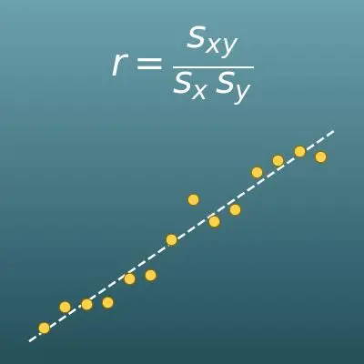
Correlation coefficient \(r\)
Figure
Standard notation (the usual math form)
\(r\) \(=\) \(s_{xy}\) \(\div\) \((\) \(s_x\) \(\times\) \(s_y\) \()\)
In words (symbols replaced with words)
④ \(r\): correlation coefficient \(=\) ① \(s_{xy}\): covariance \(\div\) \((\) ② \(s_x\): standard deviation of \(x\) \(\times\) ③ \(s_y\): standard deviation of \(y\) \()\)
The formula in words
① Divide the \(s_{xy}\): covariance
② by the product of the \(s_x\): standard deviation of \(x\)
③ and the \(s_y\): standard deviation of \(y\)
④ and you get the \(r\): correlation coefficient (\(r\) is always between \(-1\) and \(1\))
Quick example
For the same study time and score example (\(s_{xy} = 1.6\), \(s_x = \sqrt{2}\), \(s_y = \sqrt{1.6}\))
\(r\): correlation coefficient \(=\) covariance (1.6) \(\div\) \((\) \(\sqrt{2}\) \(\times\) \(\sqrt{1.6}\) \()\)
\(s_x \times s_y = \sqrt{2} \times \sqrt{1.6} = \sqrt{3.2} \approx 1.789\)
\(r = 1.6 \div 1.789 \approx 0.894\)
Key idea
The covariance is useful, but it depends on the units (just changing hours to minutes makes it 60 times larger). Dividing the covariance by the standard deviations of \(x\) and \(y\) turns it into a number from \(-1\) to \(1\) that does not depend on the units. That is the correlation coefficient \(r\). The closer \(r\) is to \(1\), the stronger the positive correlation (close to a straight line rising to the right); the closer to \(-1\), the stronger the negative correlation (close to a line falling to the right); and the closer to \(0\), the weaker the straight-line relationship. A common rule of thumb is \(0.7 \le |r|\) for a strong correlation, \(0.4 \le |r| < 0.7\) for moderate, \(0.2 \le |r| < 0.4\) for weak, and \(|r| < 0.2\) for little or no correlation (the cutoffs vary by field). Keep in mind that the correlation coefficient only measures a straight-line relationship. For a U-shaped relationship, \(r\) may be close to 0 even though there is a relationship. Also, correlation is not the same as causation (one thing causing the other).
Regression line (least squares) \(y = ax + b\)
Figure
Standard notation (the usual math form)
\(a\) \(=\) \(s_{xy}\) \(\div\) \(s_x^{2}\)
\(b\) \(=\) \(\bar{y}\) \(-\) \(a\,\bar{x}\)
In words (symbols replaced with words)
③ \(a\): slope of the regression line \(=\) ① \(s_{xy}\): covariance \(\div\) ② \(s_x^2\): variance of \(x\)
⑥ \(b\): intercept of the regression line \(=\) ④ \(\bar{y}\): mean of \(y\) \(-\) ⑤ slope \(a\) × mean of \(x\) \(\bar{x}\)
The formula in words
① Divide the \(s_{xy}\): covariance
② by the \(s_x^2\): variance of \(x\)
③ and you get the \(a\): slope of the regression line .
④ From the \(\bar{y}\): mean of \(y\)
⑤ subtract the product of the slope \(a\) and the mean of \(x\), \(\bar{x}\)
⑥ and you get the \(b\): intercept of the regression line
Quick example
For the same example (\(s_{xy} = 1.6\), \(s_x^2 = 2\), \(\bar{x} = 3\), \(\bar{y} = 4\))
slope \(a\) \(=\) covariance (1.6) \(\div\) variance of \(x\) (2)
\(a = 1.6 \div 2 = 0.8\)
\(b = 4 - 0.8 \times 3 = 1.6\)
\(y = 0.8x + 1.6\)
Key idea
The regression line is the straight line that fits the cloud of points on a scatter plot best. It is chosen so that the vertical gaps (errors) between each point and the line, squared and all added up, are as small as possible. This way of choosing the line is called the least squares method (the only arithmetic needed is the division and subtraction above). The regression line always passes through the mean point \((\bar{x},\ \bar{y})\). You can check this on the scatter plot on this page. With the regression line you can make predictions such as "with 3.5 hours of study, the score will be about \(0.8 \times 3.5 + 1.6 = 4.4\) points". But predictions that stretch the line far outside the range of the data are not reliable, and when the correlation is weak, a prediction from the line means very little. This page writes the line as \(y = ax + b\) (\(a\) is the slope, \(b\) is the intercept), the same form as LinReg(ax+b) on TI-84 calculators. In algebra it is the familiar \(y = mx + b\). Some statistics textbooks write \(\hat{y} = a + bx\) instead, with the letters for the slope and the intercept swapped.
To find the correlation coefficient: (1) find the means of \(x\) and \(y\), (2) add up all the products of deviations \((x_i - \bar{x})(y_i - \bar{y})\) and divide by the number of pairs \(n\) to get the covariance \(s_{xy}\), and (3) divide the covariance by the product of the standard deviations of \(x\) and \(y\). \(r\) is always between \(-1\) and \(1\). The closer it is to \(1\), the stronger the straight-line relationship rising to the right; the closer to \(-1\), the stronger the one falling to the right.

Symbols and terms

Symbols

\(x_i,\ y_i\) x sub i, y sub i The \(x\) value and the \(y\) value of the \(i\)th pair. (Example - the study time \(x_3\) and the score \(y_3\) of the 3rd student.) \(i\) is a letter often used for an index (position number).
\(n\) n The number of pairs, from the first letter of "number". (Example - for pairs from 5 students, \(n = 5\))
\(\bar{x},\ \bar{y}\) x-bar, y-bar The means of \(x\) and of \(y\). A bar over a letter is the customary way to show a mean.
\(x_i - \bar{x}\) x sub i minus x-bar The deviation of \(x\). It shows how far each value is from the mean of \(x\). \(y_i - \bar{y}\) is the deviation of \(y\).
\(s_{xy}\) s sub x y The covariance of \(x\) and \(y\), the mean of the products of deviations. It shows the tendency of the two sets of data to move together. The letter \(s\) is customary for statistics in the same family as the standard deviation.
\(s_x,\ s_y\) s sub x, s sub y The standard deviations of \(x\) and of \(y\) (how spread out each is). They are the square roots of the variances.
\(s_x^2,\ s_y^2\) s sub x squared, s sub y squared The variances of \(x\) and of \(y\), the mean of the squared deviations (divided by \(n\)).
\(r\) r The correlation coefficient. The letter is said to come from the \(r\) in "correlation" or "relation". It is always between \(-1\) and \(1\).
\(\sum\) sigma (summation sign) A symbol that means "add them all up". \(\sum_{i=1}^{n}\) is read "the sum from \(i = 1\) to \(n\)".
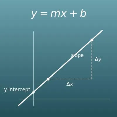
\(a,\ b\) a, b The slope and the intercept of the regression line \(y = ax + b\). They play the same roles as \(m\) and \(b\) in \(y = mx + b\).

Terms

correlation A straight-line tendency between two sets of data, where one increases as the other increases (or decreases). The stronger it is, the closer the points on a scatter plot lie to a straight line.
positive correlation The tendency for \(y\) to increase as \(x\) increases. The scatter plot rises to the right, and the correlation coefficient is positive.
negative correlation The tendency for \(y\) to decrease as \(x\) increases. The scatter plot falls to the right, and the correlation coefficient is negative.
correlation coefficient A single number from \(-1\) to \(1\) that shows the strength and direction of a correlation (also called the Pearson correlation coefficient). It is found by dividing the covariance by the product of the standard deviations of \(x\) and \(y\). Because it does not depend on the units, you can compare its strength across different data.
covariance The mean of the products of the deviations of \(x\) and \(y\). Positive means a tendency to rise to the right, and negative means a tendency to fall to the right. This page divides by the number of pairs \(n\) (the population version).
scatter plot A graph that plots paired data \((x,\ y)\) as points on a coordinate plane. From the pattern of the points you can read the direction and strength of a correlation at a glance.
variable A quantity you measure as data, such as height, score or temperature. This page looks at the relationship between two variables, \(x\) and \(y\).
deviation The difference between a value and the mean. Positive means above the mean and negative means below it. The covariance, the variance and the standard deviation are all built from deviations.
variance The mean of the squared deviations. It shows how large the spread of the data is. It appears in the denominator of the slope of the regression line.
standard deviation The square root of the variance. Its unit is the same as the data, which makes it easy to use as a measure of spread. It appears in the denominator of the correlation coefficient.
regression line (line of best fit) The straight line \(y = ax + b\) that fits the cloud of points on a scatter plot best. It is used to predict a \(y\) value from an \(x\) value.
least squares method A way to choose the slope and the intercept of a line so that the vertical gaps (errors) between each point and the line, squared and added up, are as small as possible. The regression line is the line chosen this way.
outlier A value far away from the other points. The correlation coefficient is strongly affected by outliers, so always check it together with the scatter plot.
association A relationship where two quantities move together (as one increases, the other increases or decreases). Even with a correlation, one is not necessarily the cause of the other (causation). There may simply be a common cause behind both (a third factor, also called a lurking variable).
causation (cause and effect) A relationship where one thing is the cause and the other is its result. An association (moving together) alone does not show causation; there may simply be a common cause behind both (a third factor).

Good to know before you start

Here is what helps you use the calculation on this page with real understanding, not just by pressing the button.
If you get stuck, going back to review these topics is the fastest way forward.

The mean (Grade 6)
  • Knowing that mean = sum ÷ count
  • Knowing that the mean shows roughly where the center of the data is
Negative numbers (Grades 6–7)
  • Being able to multiply with negative numbers, as in \((-1) \times 2 = -2\) and \((-2) \times (-2) = 4\)
  • Knowing that a negative times a negative is positive (this is the basis for what the sign of the covariance means)
Coordinates and linear functions (Grades 6–8)
  • Being able to plot a pair \((x,\ y)\) as a point on the coordinate plane (a scatter plot is a set of such points)
  • Knowing that in a linear function \(y = ax + b\) (like \(y = mx + b\)), \(a\) is the slope and \(b\) is the intercept (the regression line has this form)
Square roots (Grade 8)
  • Knowing a square root as "the number that gives this number when squared", as in \(\sqrt{9} = 3\)
  • Being able to multiply square roots, as in \(\sqrt{2} \times \sqrt{1.6} = \sqrt{3.2}\)
Data analysis (high school statistics)
  • Knowing what a deviation (the difference between a value and the mean) shows
  • Knowing that the variance and the standard deviation turn the size of the spread into a number (you can review them on the related Standard Deviation Calculator page)
  • Being able to read from a scatter plot whether the points rise to the right, fall to the right, or are scattered

How to calculate it in Excel

Copy the whole table below and paste it into cell A1 in Excel. It works as is.
Table to find the covariance s_xy
x of pair 1 1
x of pair 2 2
x of pair 3 3
x of pair 4 4
x of pair 5 5
y of pair 1 2
y of pair 2 4
y of pair 3 4
y of pair 4 4
y of pair 5 6
Covariance s_xy (divide by n) =COVARIANCE.P(B1:B5,B6:B10)
(For reference) sample covariance, divide by n−1 =COVARIANCE.S(B1:B5,B6:B10)
Table to find the correlation coefficient r
x of pair 1 1
x of pair 2 2
x of pair 3 3
x of pair 4 4
x of pair 5 5
y of pair 1 2
y of pair 2 4
y of pair 3 4
y of pair 4 4
y of pair 5 6
Correlation coefficient r =CORREL(B1:B5,B6:B10)
(For reference) the same value with PEARSON =PEARSON(B1:B5,B6:B10)
Table to find the regression line y = ax + b
x of pair 1 1
x of pair 2 2
x of pair 3 3
x of pair 4 4
x of pair 5 5
y of pair 1 2
y of pair 2 4
y of pair 3 4
y of pair 4 4
y of pair 5 6
Slope a =SLOPE(B6:B10,B1:B5)
Intercept b =INTERCEPT(B6:B10,B1:B5)
Table to find the means, variances and standard deviations (divide by n)
x of pair 1 1
x of pair 2 2
x of pair 3 3
x of pair 4 4
x of pair 5 5
y of pair 1 2
y of pair 2 4
y of pair 3 4
y of pair 4 4
y of pair 5 6
Mean of x x̄ =AVERAGE(B1:B5)
Mean of y ȳ =AVERAGE(B6:B10)
Variance of x s_x² =VARP(B1:B5)
Standard deviation of x s_x =STDEVP(B1:B5)
Variance of y s_y² =VARP(B6:B10)
Standard deviation of y s_y =STDEVP(B6:B10)
After pasting, B1 to B5 are the cells for x, B6 to B10 are the cells for y, and the cells in bold green are calculated automatically.
The covariance in the first table is 1.6 (the sample covariance is 2), the correlation coefficient in the second table is about 0.8944, and the third table gives a slope of 0.8 and an intercept of 1.6.
Be careful: there are two covariance functions. COVARIANCE.P is the covariance that divides by n (the same as this calculator), and COVARIANCE.S is the sample covariance that divides by n − 1. In old versions of Excel (2007 and earlier), use COVAR instead of COVARIANCE.P.
CORREL and PEARSON give the same correlation coefficient (r is the same whether you divide by n or by n − 1, so there is no choice to make).
SLOPE and INTERCEPT take "the y range, the x range" in that order (note that x does not come first).
To use a different number of pairs, add (or remove) rows of numbers, then change "B1:B5" and "B6:B10" in the formulas to your actual data ranges.

How to calculate it in Google Sheets

Copy the whole table below and paste it into cell A1 in Google Sheets. It works as is.
Table to find the covariance s_xy
x of pair 1 1
x of pair 2 2
x of pair 3 3
x of pair 4 4
x of pair 5 5
y of pair 1 2
y of pair 2 4
y of pair 3 4
y of pair 4 4
y of pair 5 6
Covariance s_xy (divide by n) =COVAR(B1:B5,B6:B10)
Table to find the correlation coefficient r
x of pair 1 1
x of pair 2 2
x of pair 3 3
x of pair 4 4
x of pair 5 5
y of pair 1 2
y of pair 2 4
y of pair 3 4
y of pair 4 4
y of pair 5 6
Correlation coefficient r =CORREL(B1:B5,B6:B10)
Table to find the regression line y = ax + b
x of pair 1 1
x of pair 2 2
x of pair 3 3
x of pair 4 4
x of pair 5 5
y of pair 1 2
y of pair 2 4
y of pair 3 4
y of pair 4 4
y of pair 5 6
Slope a =SLOPE(B6:B10,B1:B5)
Intercept b =INTERCEPT(B6:B10,B1:B5)
Almost the same functions as in Excel work as is. Copy the whole table, paste it into cell A1, and replace B1 to B10 with your own numbers.
In Google Sheets, the covariance that divides by n is found with the COVAR function (the same definition as this calculator; the name COVARIANCE.P calls the same function). The correlation coefficient uses CORREL, the same as Excel.

How to calculate it in Python

import statistics

xs = [1, 2, 3, 4, 5]      # x data (example: study time)
ys = [2, 4, 4, 4, 6]      # y data (example: quiz score)

n = len(xs)
mean_x = statistics.mean(xs)      # mean of x
mean_y = statistics.mean(ys)      # mean of y

# covariance s_xy (population version: divide by n)
covariance = sum((x - mean_x) * (y - mean_y) for x, y in zip(xs, ys)) / n

sd_x = statistics.pstdev(xs)      # standard deviation of x (divide by n)
sd_y = statistics.pstdev(ys)      # standard deviation of y (divide by n)

r = covariance / (sd_x * sd_y)    # correlation coefficient

slope = covariance / statistics.pvariance(xs)   # slope a of the regression line
intercept = mean_y - slope * mean_x             # intercept b of the regression line

print(f"Covariance s_xy: {covariance}")
print(f"Correlation coefficient r: {r}")
# the intercept can show a floating-point error (1.5999...), so round it to 10 significant digits
print(f"Regression line: y = {slope:.10g}x + {intercept:.10g}")
Runs with the standard library only (the statistics module). pstdev and pvariance, starting with "p", divide by n. When you run this example, it shows a covariance of 1.6, a correlation coefficient of 0.894… and the regression line y = 0.8x + 1.6. In Python 3.10 and later, statistics.correlation(xs, ys) gives the same correlation coefficient (r is the same whether you divide by n or by n − 1). Note that statistics.covariance(xs, ys) is the sample covariance that divides by n − 1, so to match the covariance on this page, calculate it as in the example above.

How to write it in LaTeX and other math languages (copy and paste)

Covariance \(s_{xy}\)
s_xy = {(x₁ − x̄)(y₁ − ȳ) + … + (xₙ − x̄)(yₙ − ȳ)} ÷ n
s_{xy} = \dfrac{1}{n}\sum_{i=1}^{n} (x_i - \bar{x})(y_i - \bar{y})
<math xmlns="http://www.w3.org/1998/Math/MathML" display="block">
  <mrow>
    <msub><mi>s</mi><mrow><mi>x</mi><mi>y</mi></mrow></msub>
    <mo>=</mo>
    <mfrac><mn>1</mn><mi>n</mi></mfrac>
    <munderover>
      <mo>&#x2211;</mo>
      <mrow><mi>i</mi><mo>=</mo><mn>1</mn></mrow>
      <mi>n</mi>
    </munderover>
    <mrow>
      <mo>(</mo><msub><mi>x</mi><mi>i</mi></msub><mo>&#x2212;</mo><mover><mi>x</mi><mo>&#x00AF;</mo></mover><mo>)</mo>
      <mo>(</mo><msub><mi>y</mi><mi>i</mi></msub><mo>&#x2212;</mo><mover><mi>y</mi><mo>&#x00AF;</mo></mover><mo>)</mo>
    </mrow>
  </mrow>
</math>
s_(xy) = (1/n) sum_(i=1)^n (x_i - bar x)(y_i - bar y)
Covariance[xdata, ydata]*(Length[xdata] - 1)/Length[xdata]  (* Covariance divides by n-1, so this converts it to the value divided by n *)
s_xy := add((x[i] - x_bar)*(y[i] - y_bar), i = 1 .. n)/n;
s_xy = mean((x - mean(x)).*(y - mean(y)));
s_xy = (1/n) ∑_(i=1)^n (x_i − x̄)(y_i − ȳ)
Correlation coefficient \(r\)
r = s_xy ÷ (s_x × s_y)
r = \dfrac{s_{xy}}{s_x\, s_y}
<math xmlns="http://www.w3.org/1998/Math/MathML" display="block">
  <mrow>
    <mi>r</mi>
    <mo>=</mo>
    <mfrac>
      <msub><mi>s</mi><mrow><mi>x</mi><mi>y</mi></mrow></msub>
      <mrow><msub><mi>s</mi><mi>x</mi></msub><msub><mi>s</mi><mi>y</mi></msub></mrow>
    </mfrac>
  </mrow>
</math>
r = s_(xy) / (s_x s_y)
Correlation[xdata, ydata]
r := s_xy/(s_x*s_y);
R = corrcoef(x, y); r = R(1, 2);
r = s_xy/(s_x s_y)
Regression line (least squares) \(y = ax + b\)
y = ax + b,  a = s_xy ÷ s_x²,  b = ȳ − a·x̄
y = ax + b, \quad a = \dfrac{s_{xy}}{s_x^{2}}, \quad b = \bar{y} - a\bar{x}
<math xmlns="http://www.w3.org/1998/Math/MathML" display="block">
  <mrow>
    <mi>y</mi><mo>=</mo><mi>a</mi><mi>x</mi><mo>+</mo><mi>b</mi>
    <mo>,</mo><mspace width="1em"/>
    <mi>a</mi><mo>=</mo>
    <mfrac>
      <msub><mi>s</mi><mrow><mi>x</mi><mi>y</mi></mrow></msub>
      <msubsup><mi>s</mi><mi>x</mi><mn>2</mn></msubsup>
    </mfrac>
    <mo>,</mo><mspace width="1em"/>
    <mi>b</mi><mo>=</mo>
    <mover><mi>y</mi><mo>&#x00AF;</mo></mover>
    <mo>&#x2212;</mo>
    <mi>a</mi><mover><mi>x</mi><mo>&#x00AF;</mo></mover>
  </mrow>
</math>
y = a x + b, a = s_(xy)/s_x^2, b = bar y - a bar x
lm = LinearModelFit[Transpose[{xdata, ydata}], t, t]; lm["BestFitParameters"]
a := s_xy/s_x^2; b := y_bar - a*x_bar;
p = polyfit(x, y, 1);  % p(1) = slope a, p(2) = intercept b
y = ax + b,  a = s_xy/s_x^2,  b = ȳ − ax̄

How to have ChatGPT  do the calculation

You are a statistics calculation assistant. Do the following calculation by actually running Python code, and base your answer only on the numbers from the execution result (do not answer by mental math or guessing).

For the following paired data, find each of the values below.
x: 1, 2, 3, 4, 5
y: 2, 4, 4, 4, 6
1. The means of x and y, and their variances and standard deviations dividing by n
2. The covariance s_xy (the sum of the products of deviations divided by the number of pairs n; do not divide by n − 1)
3. The correlation coefficient r
4. The slope a and the intercept b of the regression line y = ax + b (least squares)

Show the formulas you used and the numbers from the execution result.

How to Use
  1. 1
    Enter your numbers
    Type the numbers you want to calculate with into the input fields
  2. 2
    Calculate
    Press the "Calculate" button
  3. 3
    Check the result
    The result appears on the spot. The same page also explains the idea behind the calculation and the formula
  DataChef Features
Easy and Free
Unlimited conversions for free.
No technical knowledge required.
Intuitive and user-friendly operation.

No Registration Required
Available immediately after access.
Can be used without registering personal information.

Safe and Secure
Fully SSL encrypted communication.
Automatic file deletion by clicking "download".

Fast
High-speed site access
and rapid file conversion.
No Watermark
No watermark.
No attribution required.
Commercial Use Available
Free for commercial use.
No need to contact us for commercial use permission.