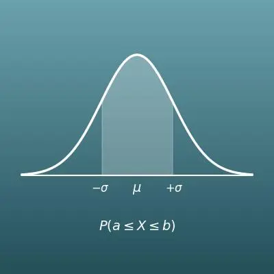
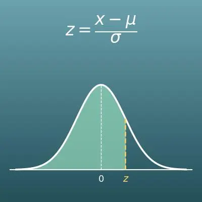
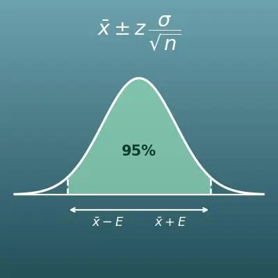
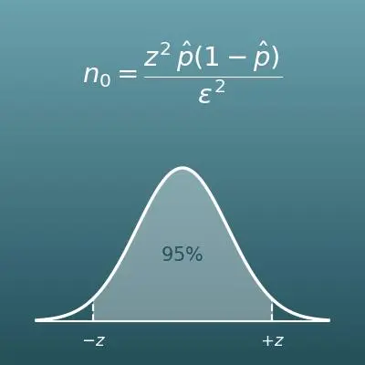










Enter the sample size, sample mean, standard deviation and confidence level. The calculator finds the confidence interval for the population mean (lower and upper bounds), the margin of error, and a table for common confidence levels.
Table of Contents
-
What you can do on this page
-
What is this calculation used for?
-
How to Use
-
Formula and graph
-
Symbols and terms
-
Good to know before you start
-
How to calculate it in Excel
-
How to calculate it in Google Sheets
-
How to calculate it in Python
-
How to write it in LaTeX and other math languages (copy and paste)
-
How to have ChatGPT do the calculation
-
DataChef Features
-
Related Features
-
NumberChef Calculators List
What you can do on this page
- Enter the sample size \(n\), the sample mean \(\bar{x}\), the standard deviation \(\sigma\) and the confidence level (%), and you get the confidence interval for the population mean (lower and upper bounds) on the spot
- It also calculates the margin of error \(E\) (how far off, plus or minus, the estimate may be), the standard error and the critical value z for the confidence level
- See the confidence intervals at common confidence levels such as 90%, 95% and 99% in one table, and check on a graph how the interval widens
- A plain-language explanation of the formulas and copy-and-paste formulas for Excel, Google Sheets and Python are all on this page
What is this calculation used for?
The "margin of error" in a poll result such as "presidential approval at 45% (margin of error ±2.5 points)" is exactly the margin of error \(E\) on this page. For a poll with 45% approval and 1,600 respondents, the spread is \(\sigma = \sqrt{0.45 \times 0.55} \approx 0.497\), so at a 95% confidence level \(E = 1.96 \times 0.497 \div \sqrt{1600} \approx 0.024\) (about ±2.4 points). This assumes the share of answers can be approximated by a normal distribution. The "±2.5 points" in news reports matches an estimate made with 50% approval, where the spread is largest.
You will be able to judge for yourself whether news that "approval moved 1 point" is within the margin of error.
A factory cannot open and measure every bottle, so it checks a sample. If 50 bottles (the standard 500 mL, or 16.9 fl oz, size) average 500.2 mL with a standard deviation of 2 mL, the 95% confidence interval for the average content of everything produced is about 499.65 to 500.75 mL.
Checking statistically, from sample inspections alone, that products are not below the labeled amount is a calculation used every day in food, beverage and drug manufacturing.
Results in medical papers are almost always reported with a confidence interval, as in "the new drug lowered blood pressure by 8.0 mmHg on average (95% confidence interval: 5.6 to 10.4)". In a 100-person study where the drops have a standard deviation of 12 mmHg, \(E = 1.96 \times 12 \div \sqrt{100} \approx 2.4\).
If the whole interval is on the plus side (it does not include 0), that supports "the drug had an effect". If the interval includes 0, read it as "it may be chance". This is one of the most important ways to read health information for yourself.
Testing every student in the country is a huge job, so national studies of fitness and achievement are often done with samples. For example, if a sample of 400 students has an average 50-meter dash time of 9.2 seconds with a standard deviation of 0.8 seconds, the 95% confidence interval for the average time of all students is about 9.12 to 9.28 seconds. Just 400 students give a fairly narrow range.
Government statistics, such as the Current Population Survey behind the monthly unemployment rate, are also based mainly on samples, and this calculation backs up how precise they are.
When the average time on your site goes up from 180 seconds to 184 seconds, is that the effect of your change, or just chance? With 2,500 visitors and a standard deviation of 90 seconds, the 95% confidence interval for the average time is about 176.5 to 183.5 seconds, so there is a range of about ±3.5 seconds.
If a change is about the same size as the width of the confidence interval, you can tell it "cannot yet be told apart from chance". This idea is the foundation for not misreading A/B test results.
Formula and graph
Symbols and terms
Symbols
| \(n\) | en | The sample size: how many items or people you actually measured. (Example: measure 50 bottles and \(n = 50\)) |
| \(\bar{x}\) | x-bar | The sample mean, the average of the sample you measured. The bar on top is the sign for an average. |
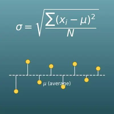
| \(\sigma\) | sigma | The population standard deviation, the size of the spread in the whole population. A Greek letter that corresponds to the English s. If the sample is large enough, the standard deviation of the sample can be used instead. |
| \(\sqrt{n}\) | square root of n | The square root of the sample size (example: \(\sqrt{25} = 5\)). It appears in the denominator of the standard error, and it is the reason 4 times the data only cuts the error in half. |
| \(z\) | zee (critical value) | The multiplier set by the confidence level. It is the boundary on the standard normal distribution that holds exactly the confidence level in the middle. For 95%, it is about 1.96. It is also written z*. |
| \(E\) | E | The margin of error. It is half the width of the confidence interval and a guide to how far, plus or minus, the sample mean may be from the population mean. E stands for "error". |
| \(L,\ U\) | L, U | The lower and upper bounds of the confidence interval, found with \(L = \bar{x} - E\) and \(U = \bar{x} + E\). |
| \(\Phi^{-1}\) | phi inverse (inverse of Φ) | The function that works the other way from \(\Phi\), the cumulative distribution function of the standard normal distribution. It takes a probability (area) and returns the matching z. (Example: \(\Phi^{-1}(0.975) \approx 1.96\)) |
| \(C\) | C | The confidence level written as a decimal. For 95%, \(C = 0.95\). |
Terms
| confidence interval | A range estimated from sample data where the population mean is likely to be. It is built by extending the sample mean up and down by the margin of error. |
| confidence level | How confident you can be in the interval. It is the share of intervals that would contain the population mean if you built intervals the same way over and over. 95% is used most often. It is also called the confidence coefficient. |
| population | The whole group you would really like to study. (Examples - every bottle a factory makes, or every voter in the country) |
| sample | The part of the population that you actually pick out and study. Using a sample to infer what the population looks like is what statistical estimation is about. |
| population mean | The mean of the whole population. You cannot measure everything, so its exact value is unknown. A confidence interval estimates where this unknown value is. It is usually written \(\mu\) (mu). |
| sample mean | The mean of the sample, \(\bar{x}\). It is the single most likely estimate of the population mean (a point estimate), but it changes a little every time depending on which sample you happen to take. |
| standard error | The size of the spread of the sample mean itself, found with \(\sigma \div \sqrt{n}\). It is easy to confuse with the spread of the individual data values (the standard deviation), so be careful. |
| interval estimate | A way to estimate an unknown value such as the population mean with a range instead of a single number. Compared with a point estimate, its strength is that it also shows how far off the estimate may be. |
| t-distribution | The distribution used instead of the normal distribution (z) when the sample is small and the population standard deviation is unknown. The calculator on this page supports only the z method. As the sample gets larger, the t-distribution gets closer to the normal distribution and the results become almost the same. |
Good to know before you start
Here is what helps you use the calculation on this page with real understanding, not just by pressing the button.
| The mean (Grade 6) |
|
| Square roots (Grade 8) |
|
| Random sampling (Grade 7) |
|
| Data analysis and standard deviation (high school statistics) |
|
| The normal distribution and interval estimates (high school statistics / AP Statistics) |
|
How to calculate it in Excel
| Confidence (%) | 95 |
| z | =NORM.S.INV((1+B1/100)/2) |
| z | 1.96 |
| Standard dev. σ | 2 |
| Sample size n | 25 |
| Margin of error E | =B1*B2/SQRT(B3) |
| Sample size n | 50 |
| Sample mean x̄ | 500.2 |
| Standard dev. σ | 2 |
| Confidence (%) | 95 |
| z | =NORM.S.INV((1+B4/100)/2) |
| Margin of error E | =B5*B3/SQRT(B1) |
| Lower bound | =B2-B6 |
| Upper bound | =B2+B6 |
The first table finds z from the confidence level (B1) alone; enter 95 and B2 is about 1.959964. The second table is the margin of error; with the example values, B4 is 0.784.
The third table finds the confidence interval from all the inputs at once. With the example values (n = 50, x̄ = 500.2, σ = 2, 95%), the lower bound (B7) is about 499.6456 and the upper bound (B8) is about 500.7544. Just replace B1 to B4 with your own numbers.
How to calculate it in Google Sheets
| Confidence (%) | 95 |
| z | =NORMSINV((1+B1/100)/2) |
| z | 1.96 |
| Standard dev. σ | 2 |
| Sample size n | 25 |
| Margin of error E | =B1*B2/SQRT(B3) |
| Sample size n | 50 |
| Sample mean x̄ | 500.2 |
| Standard dev. σ | 2 |
| Confidence (%) | 95 |
| z | =NORMSINV((1+B4/100)/2) |
| Margin of error E | =B5*B3/SQRT(B1) |
| Lower bound | =B2-B6 |
| Upper bound | =B2+B6 |
Copy the whole table, paste it into cell A1, and replace the numbers in column B with your own. The results are the same as in the Excel version: in the third table, the lower bound is about 499.6456 and the upper bound is about 500.7544.
How to calculate it in Python
import math
from statistics import NormalDist

sample_size = 50        # sample size n
sample_mean = 500.2     # sample mean x̄
sd = 2                  # standard deviation σ
confidence_level = 95   # confidence level (%)

z = NormalDist().inv_cdf((1 + confidence_level / 100) / 2)  # critical value z for the confidence level
standard_error = sd / math.sqrt(sample_size)                # standard error σ ÷ √n
margin_of_error = z * standard_error                        # margin of error E
lower = sample_mean - margin_of_error                       # lower bound of the confidence interval
upper = sample_mean + margin_of_error                       # upper bound of the confidence interval

print(f"z: {z}")
print(f"Margin of error E: {margin_of_error}")
print(f"{confidence_level}% confidence interval: {lower} to {upper}")
How to write it in LaTeX and other math languages (copy and paste)
E = z × σ ÷ √n
E = z \times \dfrac{\sigma}{\sqrt{n}}
<math xmlns="http://www.w3.org/1998/Math/MathML" display="block">
<mrow>
<mi>E</mi>
<mo>=</mo>
<mi>z</mi>
<mo>×</mo>
<mfrac>
<mi>σ</mi>
<msqrt><mi>n</mi></msqrt>
</mfrac>
</mrow>
</math>
E = z sigma / sqrt(n)
z*sigma/Sqrt[n]
E := z*sigma/sqrt(n);
E = z*sigma/sqrt(n);
E = zσ/√n
L = x̄ − E, U = x̄ + E
L = \bar{x} - E,\quad U = \bar{x} + E
<math xmlns="http://www.w3.org/1998/Math/MathML" display="block">
<mrow>
<mi>L</mi>
<mo>=</mo>
<mover><mi>x</mi><mo>¯</mo></mover>
<mo>−</mo>
<mi>E</mi>
<mo>,</mo>
<mspace width="1em"/>
<mi>U</mi>
<mo>=</mo>
<mover><mi>x</mi><mo>¯</mo></mover>
<mo>+</mo>
<mi>E</mi>
</mrow>
</math>
L = bar x - E, U = bar x + E
{xbar - e, xbar + e}
L := xbar - E; U := xbar + E;
L = xbar - E; U = xbar + E;
L = x̄ - E, U = x̄ + E
z = Φ⁻¹((1 + C) ÷ 2)
z = \Phi^{-1}\!\left(\dfrac{1+C}{2}\right)
<math xmlns="http://www.w3.org/1998/Math/MathML" display="block">
<mrow>
<mi>z</mi>
<mo>=</mo>
<msup><mi>Φ</mi><mrow><mo>−</mo><mn>1</mn></mrow></msup>
<mrow>
<mo>(</mo>
<mfrac>
<mrow><mn>1</mn><mo>+</mo><mi>C</mi></mrow>
<mn>2</mn>
</mfrac>
<mo>)</mo>
</mrow>
</mrow>
</math>
z = Phi^-1((1 + C)/2)
InverseCDF[NormalDistribution[0, 1], (1 + c)/2]
with(Statistics): Quantile(RandomVariable(Normal(0, 1)), (1 + c)/2);
z = norminv((1 + c)/2);
z = Φ^(-1)((1+C)/2)
How to have ChatGPT do the calculation
You are a statistics calculation assistant. Do the following calculation by actually running Python code, and base your answer only on the numbers from the execution result (do not answer by mental math or guessing).

50 bottles were taken off a factory line and their contents were measured. The mean was 500.2 mL. The spread of the fill amount (the population standard deviation) is known to be 2 mL.
1. Find the critical value z for a 95% confidence level (use the inverse of the cumulative distribution function of the standard normal distribution; Python's standard library statistics.NormalDist().inv_cdf can be used).
2. Find the margin of error E = z × σ ÷ √n.
3. Find the 95% confidence interval (lower and upper bounds) for the population mean (the true average content of all the bottles).

Show the formulas you used and the numbers from the execution result.
How to Use
-
1Enter your numbersType the numbers you want to calculate with into the input fields
-
2CalculatePress the "Calculate" button
-
3Check the resultThe result appears on the spot. The same page also explains the idea behind the calculation and the formula
DataChef Features

No technical knowledge required.
Intuitive and user-friendly operation.

Can be used without registering personal information.

Automatic file deletion by clicking "download".

and rapid file conversion.

No attribution required.

No need to contact us for commercial use permission.
Related Features
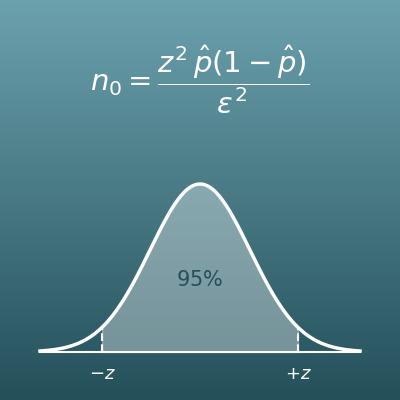
Sample Size Calculator (Surveys and Margin of Error)
From the margin of error you accept and the confidence level, work out the sample size a survey needs
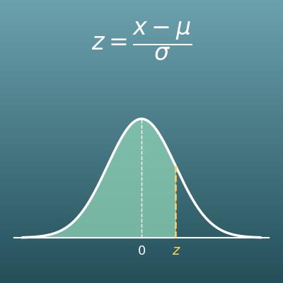
Z-Score Calculator: Z-Score to Probability and Back
Find the z-score (standard score) from a value, mean and standard deviation, and convert it to a probability and back
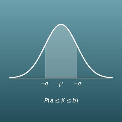
Normal Distribution Probability Calculator
From the mean and standard deviation, find the probability of falling in a given range
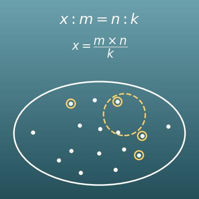
Population Estimate Calculator (Mark and Recapture, Random Samples)
The middle-school version of estimating the whole from a sample. Capture-recapture and population estimates, with the proportion worked out step by step