







Following your probability distribution table, enter each possible value x and its probability p, one row at a time. The light gray example is the prize from one raffle ticket ($0 with 70%, $1 with 20%, $5 with 9% and $100 with 1%).
Table of Contents
-
What you can do on this page
-
What is this calculation used for?
-
How to Use
-
Formulas and graph
-
Symbols and terms
-
Good to know before you start
-
How to calculate it in Excel
-
How to calculate it in Google Sheets
-
How to calculate it in Python
-
How to write it in LaTeX and other math languages (copy and paste)
-
How to have ChatGPT do the calculation
-
DataChef Features
-
Related Features
-
NumberChef Calculators List
What you can do on this page
- Enter a probability distribution table (pairs of a possible value \(x\) and its probability \(p\), 2 to 10 rows), and you get the expected value \(E(X)\), the variance \(\mathrm{Var}(X)\) and the standard deviation \(\sigma(X)\) on the spot
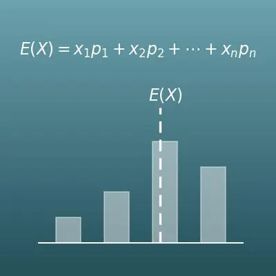
- Answers are shown both as a fraction in lowest terms (the exact value), such as \(\dfrac{7}{2}\), and as a decimal. You can also see the steps, with your numbers put into \(E(X) = x_1 p_1 + x_2 p_2 + \cdots\)
- It automatically checks that the probabilities add up to exactly 1. If they do not, it tells you what the current total is
- You can enter a probability as 0.2, 20% or 1/5. Values can also be negative (a loss)
- The result includes a bar chart of the probability distribution, with the expected value \(E(X)\) marked by a vertical dashed line
What is this calculation used for?
The expected value, "prize × chance of winning" added up over every prize, is exactly the average return per ticket. In big US lottery games such as Powerball, about half of ticket sales goes into the prize pool, so the expected value of a ticket is well below its price.
You can do the same calculation for loot boxes in video games. Using the published drop rates (probabilities), it is the basis for estimating "about how much it will cost to get the item you want".
Life and auto insurance premiums start from the expected amount paid out: "each claim payment × the chance of that accident or illness", added up. Operating costs and other amounts are then added on top. There is a whole profession, the actuary, that specializes in this kind of calculation.
From the customer's side, insurance is a deal where you pay more than you get back on average (by expected value). What you buy is peace of mind against a rare but large loss.
In investing, it is common to treat the expected value of the return (rate of return) as "the gain you can expect" and the standard deviation as "the risk (the size of the swings)". If two investments have the same expected return, the one with the smaller standard deviation moves up and down more gently.
The idea on this page, looking at "how high the expected value is" and "how big the spread is" as two separate numbers, carries straight over into real-world finance.
Board game and video game designers calculate expected values, such as "the sum of two dice", "the damage per attack" and "the value of an item from a treasure chest", to balance strength and rewards.
For example, "100 damage with a 50% chance" and "always 50 damage" both have an expected value of 50, but their variances differ, so the two moves feel different to play. Designers tune both the expected value and the spread to create the experience they want.
Formulas and graph
Symbols and terms
Symbols
| \(X\) | capital X | A random variable: a variable whose value is decided by the result of a trial, such as the number you roll on a die. Because it is a "container for a result" whose content is not yet decided, it is written with a capital letter to tell it apart from ordinary variables. |
| \(x_1,\ x_2,\ \dots,\ x_n\) | x sub 1, x sub 2, ..., x sub n | Each of the possible values of the random variable \(X\). The small number at the lower right (the subscript) only tells which value it is in the list; it has nothing to do with the value itself. |
| \(p_1,\ p_2,\ \dots,\ p_n\) | p sub 1, p sub 2, ..., p sub n | The probability of each value. \(p\) is the first letter of "probability". They always add up to 1. |
| \(n\) | n | The number of possible values (the number of rows in the probability distribution table). The letter \(n\), from "number", is often used for a count. |
| \(E(X)\) | E of X | The expected value of the random variable \(X\). \(E\) is the first letter of "expected value" (or "expectation"). It stands for one number, "the expected value of \(X\)"; it is not \(E\) times \(X\). |
| \(\mu\) | mu | The Greek letter often used for the expected value (the mean). It corresponds to "m" for "mean". Textbooks set \(\mu = E(X)\) to write the definition of the variance more compactly. |
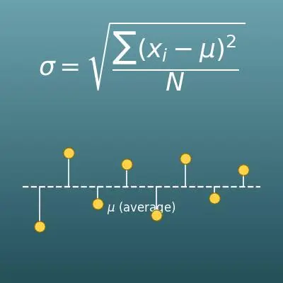
| \(\mathrm{Var}(X)\) | variance of X | The variance of the random variable \(X\). It is the average of the squared distances from the expected value (the deviations) and shows how spread out the values are. Some books write it as \(V(X)\) or \(\sigma^2\). |
| \(\sigma(X)\) | sigma of X | The standard deviation of the random variable \(X\). \(\sigma\) is the lowercase Greek letter sigma, the Greek "s" for "standard deviation". It is the positive square root of the variance. Also written \(\sigma\) or SD(X). |
| \(X^2\) | X squared | A new random variable made by squaring the value of \(X\). \(E(X^2)\) is "square each possible value first, then take the average weighted by probability". |
| \(\sqrt{\phantom{0}}\) | square root (radical sign) | The symbol for the number (0 or more) that gives the number inside when squared, the positive square root. For example, \(\sqrt{9} = 3\). The standard deviation is found by putting the variance under this symbol. |
Terms
| random variable | A variable whose value is decided by the result of a trial (an experiment or observation whose result is decided by chance), such as the number rolled on a die or the prize from a raffle ticket. It is usually written with a capital \(X\). |
| probability distribution | The list that matches each possible value of a random variable with its probability. Written as a table, it is a probability distribution table, and the input fields on this page take that table as it is. |
| trial | An experiment or observation that can be repeated under the same conditions and whose result is decided by chance, such as rolling a die or drawing a raffle ticket. |
| expected value | The mean of a random variable. It is each value times its probability, all added up, and it approaches "the average per try" when the trial is repeated many times. The symbol is \(E(X)\) or \(\mu\). |
| weighted average | An average where each value is multiplied by a "weight" before adding, instead of simply adding and dividing by the count. The expected value is a weighted average with the probabilities as the weights. |
| variance | A measure of how spread out the values are. It squares the distances from the expected value (the deviations) and averages them, weighted by probability. The symbol is \(\mathrm{Var}(X)\). |
| standard deviation | The positive square root of the variance. Unlike the variance, it is in the same units as the original values, so it is easier to compare how spread out things are. The symbol is \(\sigma(X)\). |
| deviation | The distance of a value from the expected value, \(x - \mu\). Deviations are a mix of positive and negative numbers, and their plain average is always 0, so the variance squares them before averaging. |
| law of large numbers | The rule that as you repeat a trial more and more times, the average of the actual results gets closer and closer to the expected value. It is the basis for reading the expected value as "the average per try over many repetitions". |
| discrete random variable | A random variable whose possible values are separate points (a finite number of values, or whole numbers), like the numbers on a die (1 to 6). This page handles this type. A random variable that takes continuous values, such as height, is called a continuous random variable, and its expected value is found with an integral. |
Good to know before you start
Here is what helps you use the calculation on this page with real understanding, not just by pressing the button.
If you get stuck, going back over the topics in this list is the fastest way forward.
| Basic probability (Grade 7 to high school) |
|
| Working with fractions and decimals (Grades 5–7) |
|
| The mean (Grade 6 to high school) |
|
| Squares and square roots (Grade 8) |
|
| Describing data (high school statistics) |
|
How to calculate it in Excel
| Value x₁ (losing ticket, $0) | 0 |
| Probability p₁ | 0.7 |
| Value x₂ (prize $1) | 1 |
| Probability p₂ | 0.2 |
| Value x₃ (prize $5) | 5 |
| Probability p₃ | 0.09 |
| Value x₄ (prize $100) | 100 |
| Probability p₄ | 0.01 |
| Sum of probabilities (check that it is 1) | =B2+B4+B6+B8 |
| Expected value E(X) | =B1*B2+B3*B4+B5*B6+B7*B8 |
| Value x₁ | 0 |
| Probability p₁ | 0.7 |
| Value x₂ | 1 |
| Probability p₂ | 0.2 |
| Value x₃ | 5 |
| Probability p₃ | 0.09 |
| Value x₄ | 100 |
| Probability p₄ | 0.01 |
| Expected value E(X) | =B1*B2+B3*B4+B5*B6+B7*B8 |
| Mean of the squares E(X²) | =B1^2*B2+B3^2*B4+B5^2*B6+B7^2*B8 |
| Variance Var(X) = E(X²) − [E(X)]² | =B10-B9^2 |
| Variance Var(X) | 99.7275 |
| Standard deviation σ(X) = √Var(X) | =SQRT(B1) |
The first table is the raffle example ($0 with 70%, $1 with 20%, $5 with 9% and $100 with 1%). The sum of the probabilities is 1 and the expected value is 1.65 (dollars).
The second table is the variance of the same raffle: the mean of the squares, 102.45, minus the square of the expected value, 2.7225, which is 99.7275.
The third table finds the standard deviation from that variance, about 9.99 (dollars). To add rows, add more value and probability pairs and extend the "B1*B2+…" part of the formulas in the same pattern.
How to calculate it in Google Sheets
| Value x₁ (losing ticket, $0) | 0 |
| Probability p₁ | 0.7 |
| Value x₂ (prize $1) | 1 |
| Probability p₂ | 0.2 |
| Value x₃ (prize $5) | 5 |
| Probability p₃ | 0.09 |
| Value x₄ (prize $100) | 100 |
| Probability p₄ | 0.01 |
| Sum of probabilities (check that it is 1) | =B2+B4+B6+B8 |
| Expected value E(X) | =B1*B2+B3*B4+B5*B6+B7*B8 |
| Value x₁ | 0 |
| Probability p₁ | 0.7 |
| Value x₂ | 1 |
| Probability p₂ | 0.2 |
| Value x₃ | 5 |
| Probability p₃ | 0.09 |
| Value x₄ | 100 |
| Probability p₄ | 0.01 |
| Expected value E(X) | =B1*B2+B3*B4+B5*B6+B7*B8 |
| Mean of the squares E(X²) | =B1^2*B2+B3^2*B4+B5^2*B6+B7^2*B8 |
| Variance Var(X) = E(X²) − [E(X)]² | =B10-B9^2 |
| Variance Var(X) | 99.7275 |
| Standard deviation σ(X) = √Var(X) | =SQRT(B1) |
How to calculate it in Python
from fractions import Fraction

# Probability distribution table (value and probability pairs). Raffle example: prize and chance of winning it
# A fractional probability can be written like Fraction(1, 6)
values = [Fraction(0), Fraction(1), Fraction(5), Fraction(100)]
probabilities = [Fraction("0.7"), Fraction("0.2"), Fraction("0.09"), Fraction("0.01")]

# Check that the probabilities add up to 1
total = sum(probabilities)
if total != 1:
    raise ValueError(f"The probabilities do not add up to 1 (total: {total})")

# Expected value E(X) = Σ x_i p_i
mean = sum(x * p for x, p in zip(values, probabilities))
# Mean of the squares E(X²) and variance Var(X) = E(X²) − [E(X)]²
mean_of_squares = sum(x * x * p for x, p in zip(values, probabilities))
variance = mean_of_squares - mean * mean
# Standard deviation σ(X) = √Var(X)
std_dev = float(variance) ** 0.5

print(f"Expected value E(X): {mean} = {float(mean)}")
print(f"Variance Var(X): {variance} = {float(variance)}")
print(f"Standard deviation σ(X): {std_dev}")
How to write it in LaTeX and other math languages (copy and paste)
E(X) = x₁p₁ + x₂p₂ + … + xₙpₙ
E(X) = x_1 p_1 + x_2 p_2 + \cdots + x_n p_n
<math xmlns="http://www.w3.org/1998/Math/MathML" display="block">
<mrow>
<mi>E</mi><mo>(</mo><mi>X</mi><mo>)</mo>
<mo>=</mo>
<msub><mi>x</mi><mn>1</mn></msub><msub><mi>p</mi><mn>1</mn></msub>
<mo>+</mo>
<msub><mi>x</mi><mn>2</mn></msub><msub><mi>p</mi><mn>2</mn></msub>
<mo>+</mo><mo>⋯</mo><mo>+</mo>
<msub><mi>x</mi><mi>n</mi></msub><msub><mi>p</mi><mi>n</mi></msub>
</mrow>
</math>
E(X) = x_1 p_1 + x_2 p_2 + cdots + x_n p_n
Total[x*p]
EX := add(x[i]*p[i], i = 1..n);
EX = sum(x .* p);
E(X) = x_1 p_1 + x_2 p_2 + … + x_n p_n
Var(X) = E(X²) − [E(X)]²
\mathrm{Var}(X) = E(X^{2}) - [E(X)]^{2}
<math xmlns="http://www.w3.org/1998/Math/MathML" display="block">
<mrow>
<mi>Var</mi><mo>(</mo><mi>X</mi><mo>)</mo>
<mo>=</mo>
<mi>E</mi><mo>(</mo><msup><mi>X</mi><mn>2</mn></msup><mo>)</mo>
<mo>−</mo>
<msup><mrow><mo>[</mo><mi>E</mi><mo>(</mo><mi>X</mi><mo>)</mo><mo>]</mo></mrow><mn>2</mn></msup>
</mrow>
</math>
Var(X) = E(X^2) - [E(X)]^2
Total[x^2*p] - Total[x*p]^2
VX := add(x[i]^2*p[i], i = 1..n) - EX^2;
VX = sum(x.^2 .* p) - EX^2;
Var(X) = E(X^2) - [E(X)]^2
σ(X) = √Var(X)
\sigma(X) = \sqrt{\mathrm{Var}(X)}
<math xmlns="http://www.w3.org/1998/Math/MathML" display="block">
<mrow>
<mi>σ</mi><mo>(</mo><mi>X</mi><mo>)</mo>
<mo>=</mo>
<msqrt><mi>Var</mi><mo>(</mo><mi>X</mi><mo>)</mo></msqrt>
</mrow>
</math>
sigma(X) = sqrt(Var(X))
Sqrt[Total[x^2*p] - Total[x*p]^2]
sigmaX := sqrt(VX);
sigmaX = sqrt(VX);
σ(X) = √(Var(X))
How to have ChatGPT do the calculation
You are a calculation assistant for math (probability and statistics). Do the following calculation by actually running Python code, and base your answer only on the numbers from the execution result (do not answer by mental math or guessing).

The probability distribution of a random variable X is given by this table.
Value x: 0, 1, 5, 100
Probability p: 0.7, 0.2, 0.09, 0.01

Show each of the following:
1. A check that the probabilities add up to 1
2. The expected value E(X) (both as a fraction in lowest terms or a whole number, and as a decimal)
3. The variance Var(X) (use the formula E(X²) − [E(X)]², and also show the value of E(X²))
4. The standard deviation σ(X) (as a decimal)

In Python, use the fractions module from the standard library to calculate exactly, and show the formulas you used and the numbers from the execution result.
How to Use
-
1Enter your numbersType the numbers you want to calculate with into the input fields
-
2CalculatePress the "Calculate" button
-
3Check the resultThe result appears on the spot. The same page also explains the idea behind the calculation and the formula
DataChef Features

No technical knowledge required.
Intuitive and user-friendly operation.

Can be used without registering personal information.

Automatic file deletion by clicking "download".

and rapid file conversion.

No attribution required.

No need to contact us for commercial use permission.
Related Features
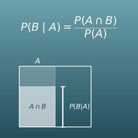
Conditional Probability and Bayes' Theorem Calculator
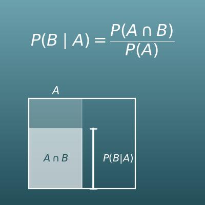
Finds P(B|A), the probability of B given that A happened, and uses Bayes' theorem to trace a result back to its cause, with an area model and a tree diagram
Probability of Repeated Trials (n in a Row, At Least Once)
Finds the probability that something with probability p happens every time, or at least once, in n trials
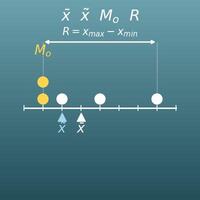
Mean, Median, Mode and Range Calculator
Enter your data to get the mean, median, mode and range at once. The mean is the "data version" of the expected value
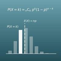
Binomial Distribution Calculator
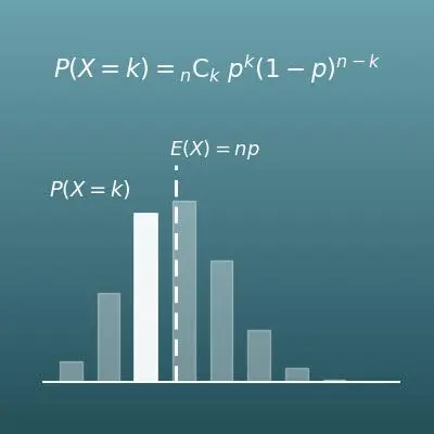
Finds the binomial mean np, the variance np(1−p) and the probability of exactly k successes in n trials, with a bar chart of the distribution