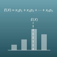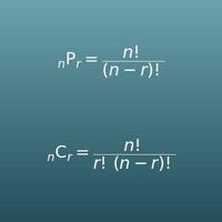































Enter the number of trials n, the probability of success on each trial p, and the number of successes k. You get the probability of exactly k successes, the cumulative probabilities of at most k and at least k, the mean, variance and standard deviation, and a bar chart of the whole distribution.
Table of Contents
-
What you can do on this page
-
What is this calculation used for?
-
How to Use
-
Formulas and graphs
-
Symbols and terms
-
Good to know before you start
-
How to calculate it in Excel
-
How to calculate it in Google Sheets
-
How to calculate it in Python
-
How to write it in LaTeX and other math languages (copy and paste)
-
How to have ChatGPT do the calculation
-
DataChef Features
-
Related Features
-
NumberChef Calculators List
What you can do on this page
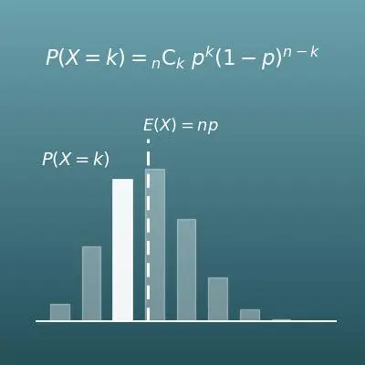
- Enter just 3 numbers to find "the probability that something with probability \(p\) happens exactly \(k\) times in \(n\) tries", \(P(X = k) = {}_{n}\mathrm{C}_{k}\, p^{k} (1-p)^{n-k}\), on the spot
- The answer is shown both as a fraction in lowest terms such as \(\dfrac{3}{8}\) (the exact value) and as a decimal and percent. You can also see the steps for the number of combinations \({}_{n}\mathrm{C}_{k}\)
- It also finds the cumulative probabilities, "at most \(k\) times" \(P(X \le k)\) and "at least \(k\) times" \(P(X \ge k)\), at the same time
- It shows the expected value \(E(X) = np\), the variance \(V(X) = np(1-p)\) and the standard deviation \(\sigma\), and checks the rule of thumb for using the normal approximation
- The whole distribution, from 0 up to \(n\) successes, is drawn as a bar chart, so you can see at a glance which counts are most likely
What is this calculation used for?
If you open 100 loot boxes (or gacha pulls) with a 1% drop rate, the number of rare drops follows the binomial distribution \(B(100,\ 0.01)\) (assuming, as published, that each try has the same chance and is independent). The chance of getting nothing at all is \(0.99^{100} \approx 36.6\%\), so the distribution shows that the gut feeling "100 tries at 1% is almost a sure thing" is risky.
Estimating "the expected value \(np\) plus the spread" when you plan how much to spend is exactly the calculation on this page.
Instead of checking every item, factories use acceptance sampling: "take \(n\) items from a lot, and accept the lot if there are \(c\) or fewer defects". The chance that a lot with a defect rate \(p\) is accepted is exactly the cumulative binomial probability \(P(X \le c)\). For example, if you take 20 items from a lot with a 1% defect rate and accept it only with 0 defects, the chance of acceptance is \(0.99^{20} \approx 81.8\%\).
This calculation is used to design inspection rules that accept good lots with high probability and reject bad ones.
If you guess on all 20 questions of a test with 4 choices each, the number of correct answers follows the binomial distribution \(B(20,\ 0.25)\), and the expected value is \(20 \times 0.25 = 5\) questions. The chance of getting 8 or more right by luck is only about 10%, which confirms with probability that guessing alone rarely reaches a passing score.
Test makers also keep this distribution in mind when they set the number of questions and the passing score, so that it is hard to pass by luck.
When a 70% free-throw shooter takes 10 shots, the chance of making exactly 7 is only \({}_{10}\mathrm{C}_{7} \times 0.7^{7} \times 0.3^{3} \approx 26.7\%\) (treating each shot as independent with a fixed success rate). A 70% shooter making exactly 7 of 10 is not as ordinary as it sounds. Making 6 or 8 happens all the time.
The binomial distribution helps you tell how much of a "hot streak" or "slump" is just normal random variation.
In approval rating polls and TV ratings, the number of people out of the \(n\) surveyed who give a certain answer is treated as following a binomial distribution. The "plus or minus a few points" margin of error is calculated from the standard deviation \(\sqrt{np(1-p)}\) and the normal approximation.
Deciding how many people to survey to get the margin of error down to a target size is based directly on the properties of the binomial distribution.
Formulas and graphs
Symbols and terms
Symbols
| \(X\) | X | The random variable for the number of successes. By convention, numbers decided by chance are written with capital letters from the end of the alphabet, such as \(X,\ Y,\ Z\). |
| \(P(X = k)\) | P of X equals k | The probability that the number of successes \(X\) is exactly \(k\). \(P\) stands for "probability". |
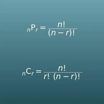
| \({}_{n}\mathrm{C}_{k}\) | n choose k | The number of combinations of \(k\) items chosen from \(n\). \(C\) stands for "combination". Many textbooks write it as \(\dbinom{n}{k}\) instead. |
| \(n\) | en | The number of trials (how many times you repeat it). The letter \(n\), for "number", is often used for counts. |
| \(p\) | pee | The probability of success on one trial. It comes from "probability", and the lowercase letter is often used for the probability of a single try. |
| \(1 - p\) | one minus p | The probability of failure on one trial (not succeeding). Either success or failure always happens, so it is what is left after subtracting \(p\) from the total of \(1\). It is also written \(q\). |
| \(k\) | kay | The number of successes, a whole number from \(0\) to \(n\). The letter \(k\) is often used to say "how many times". |
| \(P(X \le k)\) | P of X less than or equal to k | The probability of at most \(k\) successes (any of 0 through \(k\)). It is a cumulative probability, the exact probabilities added up through \(k\). |
| \(P(X \ge k)\) | P of X greater than or equal to k | The probability of at least \(k\) successes (any of \(k\) through \(n\)). Subtracting \(P(X \le k-1)\) from the total of \(1\) (the complement) shortens the sum. |
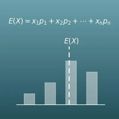
| \(E(X)\) | E of X | The expected value (the average number of successes). \(E\) stands for "expectation". For the binomial distribution, \(E(X) = np\). It is also called the mean and written \(\mu\). |
| \(V(X)\) | V of X | The variance (how spread out the results are). \(V\) stands for "variance". For the binomial distribution, \(V(X) = np(1-p)\). It is also written \(\mathrm{Var}(X)\) or \(\sigma^2\). |
| \(\sigma\) | sigma | The standard deviation. It is the lowercase Greek letter sigma, the Greek "s" as in "standard deviation". It is the square root of the variance, \(\sigma = \sqrt{V(X)}\), and shows the typical distance from the expected value. |
| \(B(n,\ p)\) | B of n, p | The binomial distribution with \(n\) trials and probability of success \(p\). \(B\) stands for "binomial". "\(X\) follows a binomial distribution" is written \(X \sim B(n,\ p)\). |
| \(N(\mu,\ \sigma^2)\) | N of mu, sigma squared | The normal distribution with mean \(\mu\) and variance \(\sigma^2\). \(N\) stands for "normal". By convention, the order inside the parentheses is "mean, variance". |
| \(\approx\) | approximately equal to | The symbol for "approximately equal". On this page it shows that the binomial distribution can be roughly replaced by the normal distribution. |
Terms
| binomial distribution | The probability distribution of "how many times something with probability \(p\) happens in \(n\) tries". The name comes from the fact that the \({}_{n}\mathrm{C}_{k}\) in the formula is the same as the binomial coefficient (the coefficients in the binomial theorem). In the US it is usually taught in high school Statistics or AP Statistics. |
| random variable | A variable whose value is decided by chance. On this page, the number of successes is the random variable. It takes the values 0 up to n, each with its own probability. |
| trial | One run of an experiment or observation whose result is decided by chance, such as one coin flip or one draw of a ticket. |
| repeated trials | Repeating the same trial with the same probability each time, where the results do not affect each other (independently). They are also called Bernoulli trials. The binomial distribution is the distribution of the number of successes in repeated trials. |
| independent | When the result of one trial does not affect the result of another. The first and second rolls of a die are independent, but drawing tickets without putting them back is not (the earlier results change how many winning tickets are left). |
| combination | A way to choose \(k\) of \(n\) items where order does not matter. The total number of them is \({}_{n}\mathrm{C}_{k}\). In the binomial distribution, it counts the ways to choose which of the \(n\) trials are successes. |
| cumulative probability | The exact probabilities added up to a certain count. The probability of at most \(k\), \(P(X \le k)\), is the typical example. |
| complement | The event that something does not happen. The probabilities always add up to 1, so a probability like "at least \(k\)" is easy to find by subtracting the opposite side (at most \(k-1\)) from 1. |
| expected value | The average value when you repeat the trials many times. For the binomial distribution it is the average number of successes, given by the simple formula \(np\). |
| variance | A measure of how far the actual values tend to be from the expected value (the spread). It is defined as the average of the squared differences. |
| standard deviation | The square root of the variance. The variance is in squared units, so taking the square root brings it back to the original unit (here, the number of successes) as a measure of spread. |
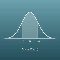
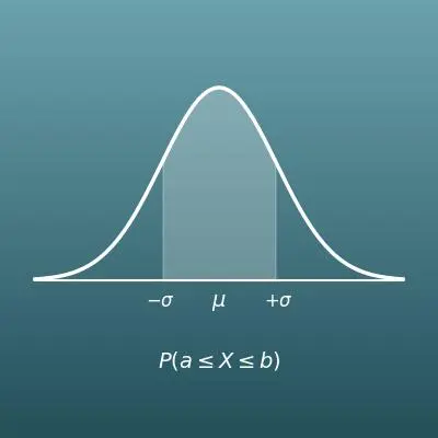
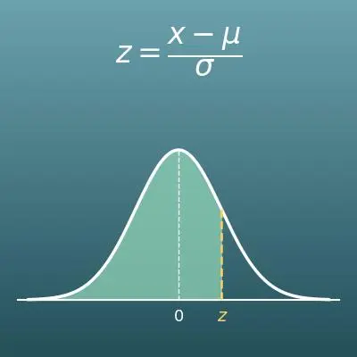
| normal distribution | A symmetric, bell-shaped distribution where values near the mean are most likely and values farther away are less likely. Many real-world quantities, such as heights and measurement errors, come close to this shape, and the binomial distribution also gets close to it when \(n\) is large. |
| normal approximation | Replacing the binomial distribution with the normal distribution \(N(np,\ np(1-p))\) when \(n\) is large. The common rule of thumb is \(np \ge 5\) and \(n(1-p) \ge 5\). |
Good to know before you start
Here is what helps you use the calculation on this page with real understanding, not just by pressing the button.
If you get stuck, going back over the topics in this table is the fastest way forward.
| Basic probability (Grade 7) |
|
| Working with fractions (Grades 5–6) |
|
| Powers and exponents (Grades 6–8, Algebra 1) |
|
| Counting and combinations (high school, Algebra 2 or Statistics) |
|
| Probability of repeated trials and the complement (high school, Statistics) |
|
| Random variables, expected value and variance (high school, AP Statistics) |
|
| The normal distribution (high school, AP Statistics) |
|
How to calculate it in Excel
| Number of trials n | 4 |
| Probability of success p | 0.5 |
| Number of successes k | 2 |
| Probability of exactly k P(X=k) | =BINOM.DIST(B3,B1,B2,FALSE) |
| Number of trials n | 4 |
| Probability of success p | 0.5 |
| Number of successes k | 2 |
| Probability of at most k P(X≤k) | =BINOM.DIST(B3,B1,B2,TRUE) |
| Probability of at least k P(X≥k) | =1-BINOM.DIST(B3-1,B1,B2,TRUE) |
| Number of trials n | 30 |
| Probability of success p | =1/6 |
| Mean E(X) = np | =B1*B2 |
| Variance V(X) = np(1-p) | =B1*B2*(1-B2) |
| Standard deviation σ | =SQRT(B4) |
| Number of trials n | 20 |
| Probability of success p | 0.5 |
| np | =B1*B2 |
| n(1-p) | =B1*(1-B2) |
| Rule of thumb met? | =AND(B3>=5,B4>=5) |
BINOM.DIST is the binomial distribution function. Its arguments are, in order, "number of successes, number of trials, probability of success, cumulative or not". FALSE at the end gives the exact probability, and TRUE gives the cumulative probability of that count or fewer.
The first table is the example of exactly 2 heads in 4 coin flips, and the answer is 0.375 (= 3/8).
Both answers in the second table are 0.6875. "At least k" is found by subtracting "at most k−1" from 1 (this formula gives an error if k is 0, but the probability of 0 or more is always 1).
The third table is the number of 1s in 30 rolls of a die: mean 5, variance 4.1667 and standard deviation 2.0412.
The fourth table shows TRUE when both np and n(1−p) are 5 or more (the rule of thumb for the normal approximation is met), and FALSE otherwise.
How to calculate it in Google Sheets
| Number of trials n | 4 |
| Probability of success p | 0.5 |
| Number of successes k | 2 |
| Probability of exactly k P(X=k) | =BINOMDIST(B3,B1,B2,FALSE) |
| Number of trials n | 4 |
| Probability of success p | 0.5 |
| Number of successes k | 2 |
| Probability of at most k P(X≤k) | =BINOMDIST(B3,B1,B2,TRUE) |
| Probability of at least k P(X≥k) | =1-BINOMDIST(B3-1,B1,B2,TRUE) |
| Number of trials n | 30 |
| Probability of success p | =1/6 |
| Mean E(X) = np | =B1*B2 |
| Variance V(X) = np(1-p) | =B1*B2*(1-B2) |
| Standard deviation σ | =SQRT(B4) |
| Number of trials n | 20 |
| Probability of success p | 0.5 |
| np | =B1*B2 |
| n(1-p) | =B1*(1-B2) |
| Rule of thumb met? | =AND(B3>=5,B4>=5) |
As in Excel, the "at least k" formula gives an error if k is 0 (the probability of 0 or more is always 1).
How to calculate it in Python
from fractions import Fraction
from math import comb, sqrt

trial_count = 4                  # number of trials n
success_prob = Fraction(1, 2)    # probability of success p (a decimal such as 0.3 also works)
success_count = 2                # number of successes k

failure_prob = 1 - success_prob

# probability of exactly k successes P(X=k) = nCk × p^k × (1−p)^(n−k)
exact_prob = (comb(trial_count, success_count)
              * success_prob ** success_count
              * failure_prob ** (trial_count - success_count))
print(f"Probability of exactly {success_count}: {exact_prob} = {float(exact_prob)}")

# cumulative probabilities (at most k, at least k)
prob_le = sum(comb(trial_count, i) * success_prob ** i * failure_prob ** (trial_count - i)
              for i in range(success_count + 1))
prob_ge = 1 - prob_le + exact_prob
print(f"Probability of at most {success_count}: {prob_le} = {float(prob_le)}")
print(f"Probability of at least {success_count}: {prob_ge} = {float(prob_ge)}")

# mean, variance and standard deviation
mean = trial_count * success_prob
variance = mean * failure_prob
print(f"Mean: {mean}  Variance: {variance}  Standard deviation: {sqrt(variance)}")
How to write it in LaTeX and other math languages (copy and paste)
P(X = k) = nCk pᵏ (1 − p)ⁿ⁻ᵏ
P(X = k) = \binom{n}{k} p^{k} (1 - p)^{n - k}
<math xmlns="http://www.w3.org/1998/Math/MathML" display="block">
<mrow>
<mi>P</mi><mo>(</mo><mi>X</mi><mo>=</mo><mi>k</mi><mo>)</mo>
<mo>=</mo>
<mrow>
<mo>(</mo>
<mfrac linethickness="0"><mi>n</mi><mi>k</mi></mfrac>
<mo>)</mo>
</mrow>
<msup><mi>p</mi><mi>k</mi></msup>
<msup>
<mrow><mo>(</mo><mn>1</mn><mo>−</mo><mi>p</mi><mo>)</mo></mrow>
<mrow><mi>n</mi><mo>−</mo><mi>k</mi></mrow>
</msup>
</mrow>
</math>
P(X = k) = C(n,k) p^k (1-p)^(n-k)
PDF[BinomialDistribution[n, p], k]
binomial(n, k)*p^k*(1-p)^(n-k);
binopdf(k, n, p)
P(X=k) = C(n,k) p^k (1-p)^(n-k)
P(X ≤ k) = Σ[i=0→k] nCi pⁱ (1 − p)ⁿ⁻ⁱ
P(X \le k) = \sum_{i=0}^{k} \binom{n}{i} p^{i} (1 - p)^{n - i}
<math xmlns="http://www.w3.org/1998/Math/MathML" display="block">
<mrow>
<mi>P</mi><mo>(</mo><mi>X</mi><mo>≤</mo><mi>k</mi><mo>)</mo>
<mo>=</mo>
<munderover>
<mo>∑</mo>
<mrow><mi>i</mi><mo>=</mo><mn>0</mn></mrow>
<mi>k</mi>
</munderover>
<mrow>
<mo>(</mo>
<mfrac linethickness="0"><mi>n</mi><mi>i</mi></mfrac>
<mo>)</mo>
</mrow>
<msup><mi>p</mi><mi>i</mi></msup>
<msup>
<mrow><mo>(</mo><mn>1</mn><mo>−</mo><mi>p</mi><mo>)</mo></mrow>
<mrow><mi>n</mi><mo>−</mo><mi>i</mi></mrow>
</msup>
</mrow>
</math>
P(X <= k) = sum_(i=0)^k C(n,i) p^i (1-p)^(n-i)
CDF[BinomialDistribution[n, p], k]
add(binomial(n, i)*p^i*(1-p)^(n-i), i = 0..k);
binocdf(k, n, p)
P(X≤k) = Σ_(i=0)^k C(n,i) p^i (1-p)^(n-i)
E(X) = np, V(X) = np(1 − p), σ = √(np(1 − p))
E(X) = np, \quad V(X) = np(1 - p), \quad \sigma = \sqrt{np(1 - p)}
<math xmlns="http://www.w3.org/1998/Math/MathML" display="block">
<mrow>
<mi>E</mi><mo>(</mo><mi>X</mi><mo>)</mo><mo>=</mo><mi>n</mi><mi>p</mi>
<mo>,</mo>
<mi>V</mi><mo>(</mo><mi>X</mi><mo>)</mo><mo>=</mo>
<mi>n</mi><mi>p</mi>
<mrow><mo>(</mo><mn>1</mn><mo>−</mo><mi>p</mi><mo>)</mo></mrow>
<mo>,</mo>
<mi>σ</mi><mo>=</mo>
<msqrt><mi>n</mi><mi>p</mi><mrow><mo>(</mo><mn>1</mn><mo>−</mo><mi>p</mi><mo>)</mo></mrow></msqrt>
</mrow>
</math>
E(X) = np, V(X) = np(1-p), sigma = sqrt(np(1-p))
{Mean[BinomialDistribution[n, p]], Variance[BinomialDistribution[n, p]], StandardDeviation[BinomialDistribution[n, p]]}
n*p; n*p*(1-p); sqrt(n*p*(1-p));
[m, v] = binostat(n, p); s = sqrt(v);
E(X) = np, V(X) = np(1-p), σ = √(np(1-p))
B(n, p) ≈ N(np, np(1 − p))
B(n,\ p) \approx N(np,\ np(1 - p))
<math xmlns="http://www.w3.org/1998/Math/MathML" display="block">
<mrow>
<mi>B</mi><mo>(</mo><mi>n</mi><mo>,</mo><mi>p</mi><mo>)</mo>
<mo>≈</mo>
<mi>N</mi><mo>(</mo><mi>n</mi><mi>p</mi><mo>,</mo>
<mi>n</mi><mi>p</mi>
<mrow><mo>(</mo><mn>1</mn><mo>−</mo><mi>p</mi><mo>)</mo></mrow>
<mo>)</mo>
</mrow>
</math>
B(n, p) ~~ N(np, np(1-p))
NormalDistribution[n p, Sqrt[n p (1 - p)]]
Normal(n*p, sqrt(n*p*(1-p)));
pd = makedist('Normal', 'mu', n*p, 'sigma', sqrt(n*p*(1-p)));
B(n, p) ≈ N(np, np(1-p))
How to have ChatGPT do the calculation
You are a calculation assistant for math (probability and statistics). Do the following calculation by actually running Python code, and base your answer only on the numbers from the execution result (do not answer by mental math or guessing).

You enter a prize draw 10 times, and each entry has a 1/6 chance of winning. For the binomial distribution of the number of wins, find:
1. The probability of winning exactly 2 times, P(X=2) (as a fraction in lowest terms and as a decimal)
2. The probability of at most 2 wins, P(X≤2), and of at least 2 wins, P(X≥2)
3. The mean E(X), variance V(X) and standard deviation σ
4. Whether the rule of thumb for the normal approximation, np ≥ 5 and n(1−p) ≥ 5, is met

In Python, calculate exactly with fractions and math.comb from the standard library, and show the formulas you used and the numbers from the execution result.
How to Use
-
1Enter your numbersType the numbers you want to calculate with into the input fields
-
2CalculatePress the "Calculate" button
-
3Check the resultThe result appears on the spot. The same page also explains the idea behind the calculation and the formula
DataChef Features

No technical knowledge required.
Intuitive and user-friendly operation.

Can be used without registering personal information.

Automatic file deletion by clicking "download".

and rapid file conversion.

No attribution required.

No need to contact us for commercial use permission.
Related Features
Probability of Repeated Trials (n in a Row, At Least Once)
Find the chance that something happens n times in a row, at least once, or never
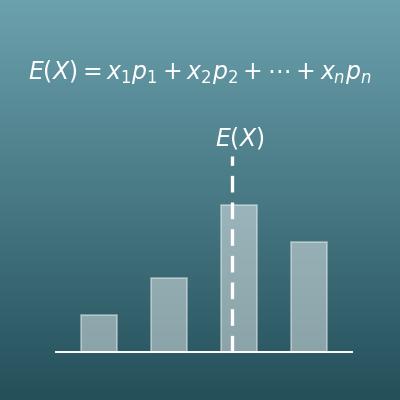
Expected Value Calculator (Mean, Variance, Standard Deviation)
Find the expected value E(X), variance V(X) and standard deviation from a probability distribution table. Works for any distribution, not just the binomial
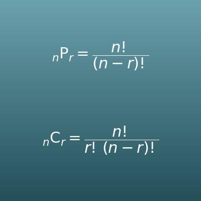
Permutation and Combination Calculator (nPr, nCr)
Calculate the number of combinations nCr (nCk) used in the binomial formula on its own, with the steps shown
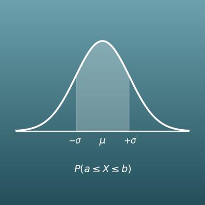
Normal Distribution Probability Calculator
From the mean and standard deviation, find the probability of falling in a given range. Use it for the normal approximation to the binomial