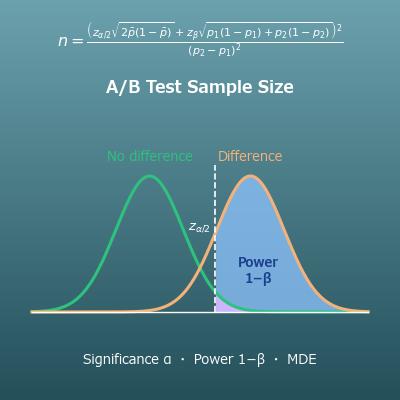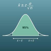






























































Enter the visitors and conversions for group A (the original version) and group B (the changed version). Along with each conversion rate, the difference and the relative lift, it runs a two-proportion z-test for the z-score and p-value, and gives a "significant / not significant" verdict at the significance level you choose.
Table of Contents
-
What you can do on this page
-
What is this calculation used for?
-
How to Use
-
Formula
-
Symbols and terms
-
Good to know before you start
-
How to calculate it in Excel
-
How to calculate it in Google Sheets
-
How to calculate it in Python
-
How to write it in LaTeX and other math languages (copy and paste)
-
How to have ChatGPT do the calculation
-
DataChef Features
-
Related Features
-
NumberChef Calculators List
What you can do on this page
- Enter the visitors (clicks or sessions also work) and conversions for groups A and B, and get each conversion rate, the difference in conversion rates and the relative lift all at once
- "B looks better, but could it just be random variation?" A two-proportion z-test answers this (z-score, two-tailed and one-tailed p-values, and a verdict at a 5%, 1% or 10% significance level)
- It also gives the confidence interval for the difference (such as 95%) and the margin by which the z-score clears (or misses) the significance line
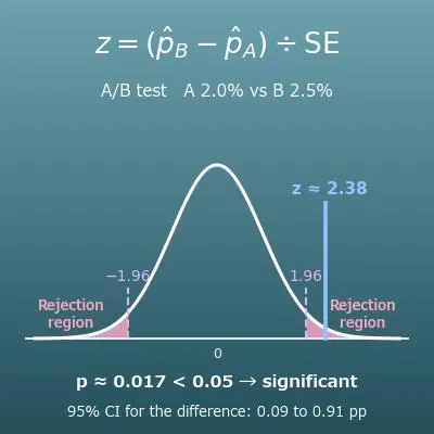
- A standard normal distribution graph shows where your z-score falls and shades the rejection region (significant if the z-score lands there)
- A plain-language explanation of the formulas and copy-and-paste formulas for Excel, Google Sheets and Python are all on this page
What is this calculation used for?
"Version B with a different button color raised the conversion rate from 2.0% to 2.5%." Checking whether this difference is not just chance is A/B test significance, done every day in online marketing. With 10,000 visitors each, the two-tailed p-value is about 0.017, "significant at 5%". But with similar conversion rates on 500 visitors each (10 conversions vs. 12 or 13), the p-value is about 0.5 to 0.7, and you can only say "it may be chance".
If you switch because "B looks better", it often happens that results drift back the next month. Deciding the number of visitors first and judging by a significance level prevents this (assuming visitors are split at random).
Send the same email with two different subject lines to half the list each and compare open rates of 48% and 52%. This is also a test of the difference between two proportions. With 5,000 emails each, the 4-point difference has a z-score of about 4, a difference that is hard to explain by chance.
Larger proportions such as open rates are easier to judge with the same number of emails than small ones such as conversion rates (the difference tends to be large compared with the standard error). This formula gives you a feel for how the metric you compare changes the number of sends you need.
Comparing improvement rates between two groups, such as "60% improved with the standard treatment and 70% with the new one", is a basic test in clinical studies (real studies use strict designs such as randomization and blinding).
Papers behind drug approvals and treatment guidelines always report p-values and confidence intervals. Once you understand this formula, you are not swayed by the single word "significant"; you can also read "how large is the difference?" and "were there enough patients?".
When a new process B seems to lower the defect rate from 1.5% to 1.0%, the verdict changes with volume: with 2,000 units each it is "within chance", and with 20,000 units each it is "a significant improvement". This calculation keeps decisions on equipment and process changes from being swayed by chance in small samples.
For small proportions like defect rates, the normal approximation gets rough when the expected number of defects (units × defect rate) falls below 5, so an exact test that uses the binomial distribution directly (such as Fisher's exact test) is chosen instead.
The same test works for comparisons such as "classes using the new textbook had a 75% pass rate, versus 65% with the old one". But if you assign textbooks by class, students were not split at random, and differences in teachers and students get mixed into the result.
In education and social science research, along with checking significance with this formula, the design matters: were groups split at random, and did anyone change how the comparison was cut after seeing the results? Knowing the assumptions behind the formula is what keeps you from being fooled by numbers.
Formula
Symbols and terms
Symbols
| \(n_A,\ n_B\) | n sub A, n sub B | Visitors (clicks or sessions) in groups A and B. \(n\) is the first letter of "number", the usual letter in statistics for sample size. |
| \(x_A,\ x_B\) | x sub A, x sub B | Conversions in groups A and B. Using \(x\) for the number of successes is the usual practice for the binomial distribution. |
| \(\hat{p}_A,\ \hat{p}_B\) | p-hat sub A, p-hat sub B | Conversion rates of groups A and B (proportions from the sample). \(p\) is the first letter of "proportion" or "probability", and the "\(\hat{}\)" (hat) on top marks a value estimated from the sample for the true value \(p\). |
| \(\hat{p}\) | p-hat | Pooled conversion rate. One estimated conversion rate from both groups combined, assuming no difference: \(\hat{p} = (x_A + x_B) \div (n_A + n_B)\). |
| \(d\) | dee | Difference in conversion rates (\(\hat{p}_B - \hat{p}_A\)), from the first letter of "difference". This page shows it times 100, in percentage points. |
| \(L\) | el | Relative lift (%), from the first letter of "lift". How many % B's conversion rate increased compared with A's. |
| \(\mathrm{SE}\) | S-E | Standard error. A guide to how much a value from the sample (here, the difference in conversion rates) moves around by chance; it is the standard deviation of that sample value. The test uses the pooled conversion rate, and the confidence interval uses \(\mathrm{SE}_d\) from each group's conversion rate. |
| \(z\) | zee | z-score (test statistic). The difference divided by the standard error: how many times the chance wobble the difference is. With no difference it follows the standard normal distribution (mean 0, standard deviation 1), so the p-value comes from how large it is. |
| \(|z|\) | absolute value of z | The size of the z-score without its sign. A two-tailed test does not care which direction the difference goes, so it uses the absolute value. |
| \(\Phi\) | phi (capital) | The cumulative distribution function of the standard normal distribution. \(\Phi(z)\) is the probability that a standard normal value is \(z\) or less, the area under the bell curve to the left of \(z\). The Greek capital letter phi is the usual symbol for it. |
| \(p_2,\ p_1\) | p sub 2, p sub 1 | The two-tailed and one-tailed p-values. The subscripts 2 and 1 stand for "two tails" and "one tail", a labeling used on this page only; statistics textbooks just write \(p\). |
| \(\alpha\) | alpha | The significance level: the line set in advance where "if the p-value is smaller, reject the null hypothesis". 5% (0.05) is common. Greek letter alpha; it is the probability of a Type I error (calling a difference real when there is none). |
| \(z_{\alpha/2}\) | z sub alpha over 2 | The boundary z-score (critical value) that leaves a total probability of \(\alpha\) in the two tails. 1.96 for a 95% confidence interval (\(\alpha = 0.05\)) and 2.576 for 99%. For one tail it is \(z_\alpha\) (1.645 for 5%). |
| \(d_L,\ d_U\) | d sub L, d sub U | The lower and upper limits of the confidence interval for the difference: the two ends of the range where the true difference is likely to be. |
Terms
| A/B test | An experiment that shows visitors the original version (A) or a changed version (B) at random over the same period and compares the results. Widely used for websites, ads and email. Splitting at random makes factors other than the version (day of the week, traffic source and so on) the same in both groups. |
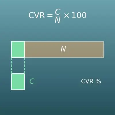
| conversion rate (CVR) | The share of visits (clicks) that led to a result (conversion) such as a purchase or sign-up. To calculate or work back from a single conversion rate, see the conversion rate calculator page. |
| null hypothesis | The hypothesis the test tries to reject: "A and B really have the same conversion rate" (\(p_A = p_B\)). The test checks how unlikely the observed difference would be if this were true. |
| alternative hypothesis | The hypothesis you want to show, opposite to the null hypothesis. In a two-tailed test it is "A and B differ" (\(p_A \neq p_B\)); in a one-tailed test, "B is higher than A" (\(p_B > p_A\)). |
| significance level | The line set before the test - if the p-value is smaller, reject the null hypothesis. 5% is common; use 1% for a stricter test. "Significant at 5%" says "the chance of a difference this large with no real difference is under 5%". |
| p-value | The probability of a difference at least this large arising by chance, assuming the null hypothesis (no difference) is true. The smaller it is, the harder the result is to explain by chance. Note that it is not "the probability that B is better" (a common misunderstanding). |
| statistically significant | The p-value is below the significance level, so the difference is judged hard to explain by random variation. It does not promise that the difference is large or the effect certain; with a huge number of visitors, even a tiny difference becomes significant. |
| test statistic | A single number calculated from the data for the test. On this page it is the z-score, "difference ÷ standard error". How extreme it is decides the p-value. |
| two-proportion z-test | A test that uses the normal distribution to check whether the proportions (such as conversion rates) of two groups differ. It is the most basic way to judge A/B test significance. You can do almost the same thing with a 2×2 chi-square test, and the two-tailed p-values match. |
| standard error | The standard deviation of a statistic from a sample (here, the difference in conversion rates) - how much it moves around by chance depending on the sample. It shrinks in proportion to the square root of the visitors, so halving the standard error takes 4 times as many visitors. |
| pooling | Combining both groups' data into one conversion rate estimate, on the assumption that there is no difference. The standard error for the test uses this pooled value. |
| confidence interval | The range where the true difference is likely to be. A 95% confidence interval is a way of building intervals so that, if you repeated the experiment many times, 95% of them would contain the true difference. If the interval does not include 0, that almost always agrees with significance in a two-tailed test at 5%. |
| two-tailed test | A test of "is there a difference (whichever is higher)?". Use it for an ordinary A/B test where you do not know which way it will go. |
| one-tailed test | A test with a fixed direction, such as "is B higher than A?". Its p-value is half the two-tailed one, so it becomes significant more easily; use it only if you decided the direction before the test. |
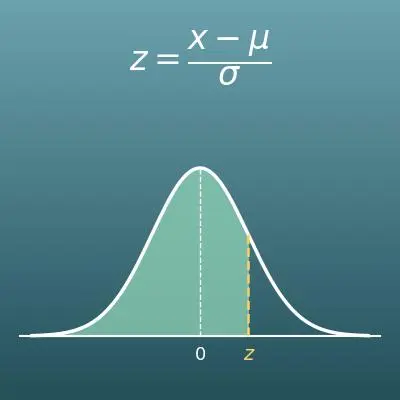
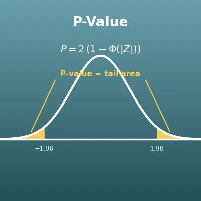
| rejection region | The tail area of the standard normal distribution where, if the z-score lands there, you reject the null hypothesis. For two-tailed 5% it is the two tails \(z < -1.96\) and \(z > 1.96\), with a total area of 0.05. It is the shaded part of the graph on this page. |
| critical value | The z-score at the edge of the rejection region. 1.96 for two-tailed 5%, 2.576 for two-tailed 1% and 1.645 for one-tailed 5%. The "z-score margin" in the result shows how far this z-score is above (or below) the critical value. |
| normal approximation | Conversion counts really follow a binomial distribution, but with many visitors a normal distribution (bell curve) approximates it well. The z-test uses this approximation, so as a guide the expected conversions \(n\hat{p}\) and expected non-conversions \(n(1-\hat{p})\) in each group should be 5 or more (10 or more if possible). |
| statistical power | The probability that the test detects a real difference as significant. With few visitors, power is low, and even a real effect often comes out "not significant". "Not significant" does not prove "no difference". |
| Type I error | Calling a result significant when there is really no difference (a false positive). The significance level \(\alpha\) is the chance of this error you accept; at 5%, "run 100 tests with no real difference and about 5 will be significant by chance". |
| multiple comparisons | Testing many versions or metrics at once. Even at a 5% significance level, test 20 metrics and one will likely be "significant" by chance. You need to narrow the metrics in advance or use a stricter significance level (Bonferroni correction and others). |
| peeking (stopping early) | Checking the results again and again during the test and stopping as soon as it looks significant. The p-value goes up and down during a test, so if you keep "stopping the first time it drops below 5%", the chance of significance with no real difference goes far above 5%. The basic rule is to decide the visitors needed first and wait until you reach them. |
| relative lift | How many % B's conversion rate increased compared with A's: the difference \(d\) divided by A's conversion rate, times 100. "Up 25%" is easier to turn into estimates of extra conversions and revenue than "up 0.5 points". |
| percentage point | The unit for the result of subtracting one percentage from another (abbreviated pp). Used as in "2.5% − 2% = 0.5 percentage points"; writing "0.5%" could be mistaken for "0.5% of 2%". |
Good to know before you start
Here is what helps you use the calculation on this page with real understanding, not just by pressing the button.
If you get stuck, going back over these topics is the quickest way forward.
| Percents (Grades 6–7) |
|
| Reciprocals and square roots (Grades 6–8) |
|
| The normal distribution and standard deviation (high school statistics, AP Statistics) |
|
| The logic of hypothesis testing (high school statistics, AP Statistics) |
|
| The binomial distribution and its normal approximation (AP Statistics) |
|
How to calculate it in Excel
| Visitors in A n_A | 10000 |
| Conversions in A x_A | 200 |
| Visitors in B n_B | 10000 |
| Conversions in B x_B | 250 |
| Conversion rate of A p̂_A | =B2/B1 |
| Conversion rate of B p̂_B | =B4/B3 |
| Conversion rate of A p̂_A | 0.02 |
| Conversion rate of B p̂_B | 0.025 |
| Difference d | =B2-B1 |
| Relative lift L (%) | =B3/B1*100 |
| Conversions in A x_A | 200 |
| Conversions in B x_B | 250 |
| Visitors in A n_A | 10000 |
| Visitors in B n_B | 10000 |
| Pooled conversion rate p̂ | =(B1+B2)/(B3+B4) |
| Pooled conversion rate p̂ | 0.0225 |
| Visitors in A n_A | 10000 |
| Visitors in B n_B | 10000 |
| Difference d | 0.005 |
| Standard error SE | =SQRT(B1*(1-B1)*(1/B2+1/B3)) |
| z-score z | =B4/B5 |
| z-score z | 2.384 |
| Two-tailed p-value p₂ | =2*(1-NORM.S.DIST(ABS(B1),TRUE)) |
| One-tailed p-value p₁ | =1-NORM.S.DIST(B1,TRUE) |
| Conversion rate of A p̂_A | 0.02 |
| Visitors in A n_A | 10000 |
| Conversion rate of B p̂_B | 0.025 |
| Visitors in B n_B | 10000 |
| Difference d | 0.005 |
| Confidence level (0.95 = 95%) | 0.95 |
| z_(α/2) | =NORM.S.INV(1-(1-B6)/2) |
| Standard error SE_d | =SQRT(B1*(1-B1)/B2+B3*(1-B3)/B4) |
| Lower limit d_L | =B5-B7*B8 |
| Upper limit d_U | =B5+B7*B8 |
In the first table, B5 shows A's conversion rate 0.02 and B6 shows B's 0.025. The second table gives a difference of 0.005 (0.5 percentage points) and a lift of 25, the third a pooled conversion rate of 0.0225, and the fourth a standard error of about 0.002097 and a z-score of about 2.384.
In the fifth table, NORM.S.DIST(z, TRUE) returns the standard normal cumulative probability Φ(z); the two-tailed p-value is about 0.0171 and the one-tailed p-value about 0.0086. In the sixth table, NORM.S.INV finds the z-score from a cumulative probability (1.96 for a 95% confidence level), giving a lower limit of about 0.0009 and an upper limit of about 0.0091 (0.09 to 0.91 percentage points).
How to calculate it in Google Sheets
| Visitors in A n_A | 10000 |
| Conversions in A x_A | 200 |
| Visitors in B n_B | 10000 |
| Conversions in B x_B | 250 |
| Conversion rate of A p̂_A | =B2/B1 |
| Conversion rate of B p̂_B | =B4/B3 |
| Conversion rate of A p̂_A | 0.02 |
| Conversion rate of B p̂_B | 0.025 |
| Difference d | =B2-B1 |
| Relative lift L (%) | =B3/B1*100 |
| Conversions in A x_A | 200 |
| Conversions in B x_B | 250 |
| Visitors in A n_A | 10000 |
| Visitors in B n_B | 10000 |
| Pooled conversion rate p̂ | =(B1+B2)/(B3+B4) |
| Pooled conversion rate p̂ | 0.0225 |
| Visitors in A n_A | 10000 |
| Visitors in B n_B | 10000 |
| Difference d | 0.005 |
| Standard error SE | =SQRT(B1*(1-B1)*(1/B2+1/B3)) |
| z-score z | =B4/B5 |
| z-score z | 2.384 |
| Two-tailed p-value p₂ | =2*(1-NORMSDIST(ABS(B1))) |
| One-tailed p-value p₁ | =1-NORMSDIST(B1) |
| Conversion rate of A p̂_A | 0.02 |
| Visitors in A n_A | 10000 |
| Conversion rate of B p̂_B | 0.025 |
| Visitors in B n_B | 10000 |
| Difference d | 0.005 |
| Confidence level (0.95 = 95%) | 0.95 |
| z_(α/2) | =NORMSINV(1-(1-B6)/2) |
| Standard error SE_d | =SQRT(B1*(1-B1)/B2+B3*(1-B3)/B4) |
| Lower limit d_L | =B5-B7*B8 |
| Upper limit d_U | =B5+B7*B8 |
How to calculate it in Python
import math

visits_a, conversions_a = 10000, 200   # visitors and conversions in A
visits_b, conversions_b = 10000, 250   # visitors and conversions in B
alpha = 0.05                           # significance level (5%)

def normal_cdf(z):
    # standard normal cumulative distribution function Φ(z)
    return 0.5 * math.erfc(-z / math.sqrt(2))

def normal_ppf(p):
    # inverse of Φ (bisection; used to find z_(α/2))
    low, high = -10.0, 10.0
    for _ in range(100):
        mid = (low + high) / 2
        if normal_cdf(mid) < p:
            low = mid
        else:
            high = mid
    return (low + high) / 2

cvr_a = conversions_a / visits_a
cvr_b = conversions_b / visits_b
diff = cvr_b - cvr_a
lift = diff / cvr_a * 100
pooled = (conversions_a + conversions_b) / (visits_a + visits_b)
se_pooled = math.sqrt(pooled * (1 - pooled) * (1 / visits_a + 1 / visits_b))
z = diff / se_pooled
p_two_sided = 2 * (1 - normal_cdf(abs(z)))
p_one_sided = 1 - normal_cdf(z)

se_diff = math.sqrt(cvr_a * (1 - cvr_a) / visits_a + cvr_b * (1 - cvr_b) / visits_b)
z_half = normal_ppf(1 - alpha / 2)
ci_low, ci_high = diff - z_half * se_diff, diff + z_half * se_diff

print(f"Conversion rate A: {cvr_a * 100:.2f}%  Conversion rate B: {cvr_b * 100:.2f}%")
print(f"Difference: {diff * 100:.2f} percentage points  Relative lift: {lift:.1f}%")
print(f"z-score: {z:.3f}  two-tailed p-value: {p_two_sided:.4f}  one-tailed p-value: {p_one_sided:.4f}")
print("Verdict (two-tailed):", "statistically significant" if p_two_sided < alpha else "not statistically significant")
print(f"{(1 - alpha) * 100:.0f}% confidence interval for the difference: {ci_low * 100:.2f} to {ci_high * 100:.2f} percentage points")
How to write it in LaTeX and other math languages (copy and paste)
p̂_A = x_A ÷ n_A
\hat{p}_A = \dfrac{x_A}{n_A}
<math xmlns="http://www.w3.org/1998/Math/MathML" display="block">
  <mrow>
    <msub><mover accent="true"><mi>p</mi><mo>^</mo></mover><mi>A</mi></msub>
    <mo>=</mo>
    <mfrac>
      <msub><mi>x</mi><mi>A</mi></msub>
      <msub><mi>n</mi><mi>A</mi></msub>
    </mfrac>
  </mrow>
</math>
hat(p)_A = x_A / n_A
xA/nA
pA := xA/nA;
pA = xA/nA;
p̂_A = x_A/n_A
d = p̂_B − p̂_A, L = d ÷ p̂_A × 100
d = \hat{p}_B - \hat{p}_A, \quad L = \dfrac{d}{\hat{p}_A} \times 100
<math xmlns="http://www.w3.org/1998/Math/MathML" display="block">
<mrow>
<mi>d</mi><mo>=</mo>
<msub><mover accent="true"><mi>p</mi><mo>^</mo></mover><mi>B</mi></msub>
<mo>−</mo>
<msub><mover accent="true"><mi>p</mi><mo>^</mo></mover><mi>A</mi></msub>
<mo>,</mo><mspace width="1em"/>
<mi>L</mi><mo>=</mo>
<mfrac><mi>d</mi><msub><mover accent="true"><mi>p</mi><mo>^</mo></mover><mi>A</mi></msub></mfrac>
<mo>×</mo><mn>100</mn>
</mrow>
</math>
d = hat(p)_B - hat(p)_A, L = d / hat(p)_A xx 100
d = pB - pA; d/pA*100
d := pB - pA; L := d/pA*100;
d = pB - pA; L = d/pA*100;
d = p̂_B − p̂_A, L = d/p̂_A × 100
p̂ = (x_A + x_B) ÷ (n_A + n_B)
\hat{p} = \dfrac{x_A + x_B}{n_A + n_B}
<math xmlns="http://www.w3.org/1998/Math/MathML" display="block">
  <mrow>
    <mover accent="true"><mi>p</mi><mo>^</mo></mover>
    <mo>=</mo>
    <mfrac>
      <mrow><msub><mi>x</mi><mi>A</mi></msub><mo>+</mo><msub><mi>x</mi><mi>B</mi></msub></mrow>
      <mrow><msub><mi>n</mi><mi>A</mi></msub><mo>+</mo><msub><mi>n</mi><mi>B</mi></msub></mrow>
    </mfrac>
  </mrow>
</math>
hat(p) = (x_A + x_B) / (n_A + n_B)
(xA + xB)/(nA + nB)
pPool := (xA + xB)/(nA + nB);
pPool = (xA + xB)/(nA + nB);
p̂ = (x_A + x_B)/(n_A + n_B)
SE = √(p̂(1 − p̂)(1/n_A + 1/n_B)), z = d ÷ SE
\mathrm{SE} = \sqrt{\hat{p}(1-\hat{p})\left(\dfrac{1}{n_A}+\dfrac{1}{n_B}\right)}, \quad z = \dfrac{d}{\mathrm{SE}}
<math xmlns="http://www.w3.org/1998/Math/MathML" display="block">
<mrow>
<mi>z</mi><mo>=</mo>
<mfrac>
<mrow><msub><mover accent="true"><mi>p</mi><mo>^</mo></mover><mi>B</mi></msub><mo>−</mo><msub><mover accent="true"><mi>p</mi><mo>^</mo></mover><mi>A</mi></msub></mrow>
<msqrt>
<mover accent="true"><mi>p</mi><mo>^</mo></mover>
<mo>(</mo><mn>1</mn><mo>−</mo><mover accent="true"><mi>p</mi><mo>^</mo></mover><mo>)</mo>
<mo>(</mo>
<mfrac><mn>1</mn><msub><mi>n</mi><mi>A</mi></msub></mfrac>
<mo>+</mo>
<mfrac><mn>1</mn><msub><mi>n</mi><mi>B</mi></msub></mfrac>
<mo>)</mo>
</msqrt>
</mfrac>
</mrow>
</math>
SE = sqrt(hat(p)(1 - hat(p))(1/n_A + 1/n_B)), z = d / SE
se = Sqrt[pPool*(1 - pPool)*(1/nA + 1/nB)]; z = d/se
SE := sqrt(pPool*(1 - pPool)*(1/nA + 1/nB)); z := d/SE;
SE = sqrt(pPool*(1 - pPool)*(1/nA + 1/nB)); z = d/SE;
SE = √(p̂(1 − p̂)(1/n_A + 1/n_B)), z = d/SE
p₂ = 2(1 − Φ(|z|)), p₁ = 1 − Φ(z)
p_2 = 2\left(1 - \Phi(|z|)\right), \quad p_1 = 1 - \Phi(z)
<math xmlns="http://www.w3.org/1998/Math/MathML" display="block">
<mrow>
<msub><mi>p</mi><mn>2</mn></msub><mo>=</mo>
<mn>2</mn><mo>(</mo><mn>1</mn><mo>−</mo>
<mi>Φ</mi><mo>(</mo><mo>|</mo><mi>z</mi><mo>|</mo><mo>)</mo><mo>)</mo>
<mo>,</mo><mspace width="1em"/>
<msub><mi>p</mi><mn>1</mn></msub><mo>=</mo>
<mn>1</mn><mo>−</mo><mi>Φ</mi><mo>(</mo><mi>z</mi><mo>)</mo>
</mrow>
</math>
p_2 = 2(1 - Phi(|z|)), p_1 = 1 - Phi(z)
p2 = 2*(1 - CDF[NormalDistribution[0, 1], Abs[z]]); p1 = 1 - CDF[NormalDistribution[0, 1], z]
p2 := 2*(1 - Statistics:-CDF(Normal(0, 1), abs(z))); p1 := 1 - Statistics:-CDF(Normal(0, 1), z);
p2 = 2*(1 - normcdf(abs(z))); p1 = 1 - normcdf(z);
p_2 = 2(1 − Φ(|z|)), p_1 = 1 − Φ(z)
d ± z_(α/2) × √(p̂_A(1 − p̂_A)/n_A + p̂_B(1 − p̂_B)/n_B)
d \pm z_{\alpha/2}\sqrt{\dfrac{\hat{p}_A(1-\hat{p}_A)}{n_A}+\dfrac{\hat{p}_B(1-\hat{p}_B)}{n_B}}
<math xmlns="http://www.w3.org/1998/Math/MathML" display="block">
<mrow>
<mi>d</mi><mo>±</mo>
<msub><mi>z</mi><mrow><mi>α</mi><mo>/</mo><mn>2</mn></mrow></msub>
<msqrt>
<mfrac>
<mrow><msub><mover accent="true"><mi>p</mi><mo>^</mo></mover><mi>A</mi></msub><mo>(</mo><mn>1</mn><mo>−</mo><msub><mover accent="true"><mi>p</mi><mo>^</mo></mover><mi>A</mi></msub><mo>)</mo></mrow>
<msub><mi>n</mi><mi>A</mi></msub>
</mfrac>
<mo>+</mo>
<mfrac>
<mrow><msub><mover accent="true"><mi>p</mi><mo>^</mo></mover><mi>B</mi></msub><mo>(</mo><mn>1</mn><mo>−</mo><msub><mover accent="true"><mi>p</mi><mo>^</mo></mover><mi>B</mi></msub><mo>)</mo></mrow>
<msub><mi>n</mi><mi>B</mi></msub>
</mfrac>
</msqrt>
</mrow>
</math>
d +- z_(alpha/2) sqrt((hat(p)_A(1 - hat(p)_A))/n_A + (hat(p)_B(1 - hat(p)_B))/n_B)
seD = Sqrt[pA*(1 - pA)/nA + pB*(1 - pB)/nB]; {d - zHalf*seD, d + zHalf*seD}
seD := sqrt(pA*(1 - pA)/nA + pB*(1 - pB)/nB); [d - zHalf*seD, d + zHalf*seD];
seD = sqrt(pA*(1 - pA)/nA + pB*(1 - pB)/nB); ci = [d - zHalf*seD, d + zHalf*seD];
d ± z_(α/2) √(p̂_A(1 − p̂_A)/n_A + p̂_B(1 − p̂_B)/n_B)
How to have ChatGPT do the calculation
You are a calculation assistant for statistics (hypothesis testing). Do the following calculation by actually running Python code, and base your answer only on the numbers from the execution result (do not answer by mental math or guessing).

The A/B test results are:
- Group A: 10000 visitors, 200 conversions
- Group B: 10000 visitors, 250 conversions
Find each of the following:
1. The conversion rate of each group (%), the difference in conversion rates (percentage points) and the relative lift (%)
2. The pooled conversion rate and the pooled standard error SE = √(p̂(1−p̂)(1/n_A + 1/n_B))
3. The z-score = difference ÷ SE, and the two-tailed and one-tailed p-values (standard normal distribution)
4. Whether the difference is statistically significant at a 5% significance level (two-tailed)
5. The 95% confidence interval for the difference (using the standard error from each group's conversion rate, √(p̂_A(1−p̂_A)/n_A + p̂_B(1−p̂_B)/n_B))

In Python, use math.erfc (or scipy.stats.norm) and show the formulas you used and the numbers from the execution result.
How to Use
-
1Enter your numbersType the numbers you want to calculate with into the input fields
-
2CalculatePress the "Calculate" button
-
3Check the resultThe result appears on the spot. The same page also explains the idea behind the calculation and the formula
DataChef Features

No technical knowledge required.
Intuitive and user-friendly operation.

Can be used without registering personal information.

Automatic file deletion by clicking "download".

and rapid file conversion.

No attribution required.

No need to contact us for commercial use permission.
Related Features
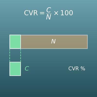
Conversion Rate Calculator (CVR, Visitors Needed and Expected Conversions)
Enter two of visits, conversions and conversion rate to get the third. Use it if you only need the conversion rate of one group
P-Value Calculator: Z-Score to P-Value and Back
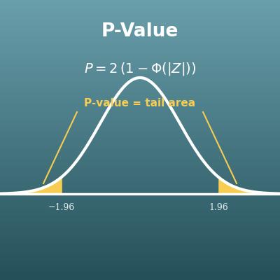
A general calculator that converts a z-score you already have into a left-tailed, right-tailed or two-tailed p-value. This page starts one step earlier, from visitors and conversions
Confidence Interval Calculator for a Population Mean
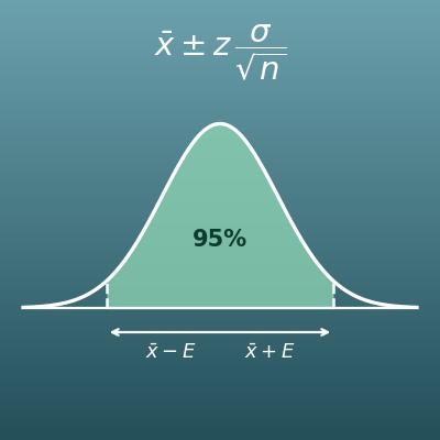
Finds the confidence interval for an average (test scores, sales and so on). The average-value version of the confidence interval for the difference on this page
Sample Size Calculator (Surveys and Margin of Error)
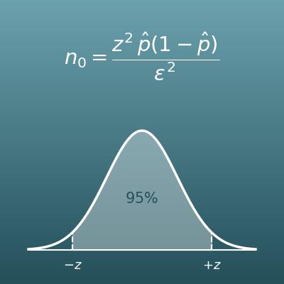
Calculates the number of people needed to estimate one proportion within a margin of error in a survey. Use it to design surveys