






















































To find the sample size, enter the baseline CVR, the MDE, the significance level and the power, then press "Calculate". You get the sample size per group for A and B (rounded up) and the total, plus the days needed if you enter your daily visitors. Switch "Solve for" to power to fix the sample size per group and find the power 1 − β instead.
Table of Contents
-
What you can do on this page
-
What is this calculation used for?
-
How to Use
-
Formulas and figures
-
Symbols and terms
-
Good to know before you start
-
How to calculate it in Excel
-
How to calculate it in Google Sheets
-
How to calculate it in Python
-
How to write it in LaTeX and other math languages (copy and paste)
-
How to have ChatGPT do the calculation
-
DataChef Features
-
Related Features
-
NumberChef Calculators List
What you can do on this page
- Enter the baseline CVR (the conversion rate of your current version A), the minimum detectable effect (MDE, as a relative % or in percentage points), the significance level \(\alpha\) (two-sided or one-sided) and the power \(1-\beta\). You get the sample size each group of your A/B test needs (rounded up) and the total
- "My page converts at 3%. How many visitors do A and B each need to detect a 10% lift (3% to 3.3%)?" This page answers the most important question to ask before a test starts
- Enter your daily visitors (optional) to also see how many days it takes to reach that sample size (rounded up)
- If you can only get a fixed number of visitors per group, fix the sample size and solve for the power \(1-\beta\) (the chance of finding a difference when there really is one)
- A graph of how the sample size changes with the MDE, a plain-language explanation of the formulas, and copy-and-paste formulas for Excel, Google Sheets and Python are all on this page
What is this calculation used for?
Suppose an online store's product page converts at 2%, and you want to detect a relative lift of 10% (2% to 2.2%) from new button text. With a 5% significance level (two-sided) and 80% power, you need about 80,682 visitors per group, about 161,364 in total.
Comparing a few dozen or a few hundred visitors ("B did better last week") cannot tell a chance difference from a real one. Working out the sample size before you start keeps you from spending weeks on a test that cannot give an answer.
A landing page gets demo requests at a 5% CVR. To detect a 1-point lift (5% to 6%), you need 8,158 visitors per group, 16,316 in total. At 300 visits a day, that is \(16316 \div 300 \approx 54.4\), so 55 days, or 8 weeks if you want to even out the days of the week.
If someone asks for results in 2 weeks, this calculation lets you explain with numbers: "In 2 weeks (4,200 visitors, 2,100 per group), we would need a much larger MDE, around 3 points (5% to 8%, which needs 1,059 per group)."
If your newsletter has a 20% open rate and you want to detect a 2-point lift (20% to 22%) from a new subject line, you need to send to 6,510 people per group, 13,020 in total (5% significance level, 80% power).
A metric with a high rate, like an open rate, needs fewer people to show a difference than a CVR of a few percent. This is because the \(p(1-p)\) part of the formula is different: the same "2 points" needs a different sample size for each metric.
Suppose a test aimed at a relative 10% lift on a page with a 3% CVR ran with 5,000 visitors per group and showed "no significant difference". Working back the power gives only about 13.5%. The test was set up to miss a real improvement more than 8 times out of 10.
The right conclusion here is not "it had no effect" but "this sample size could not tell". Working back the power keeps you from misreading a test and throwing away a good idea.
An app has a 40% next-day retention rate. To detect a relative 10% lift (40% to 44%) from a new tutorial, about 2,389 new users per group, about 4,778 in total, are enough (5% significance level, 80% power).
A metric close to 50%, like retention, has a large spread, but the difference in rates (4 points) is also large, so results come faster than in a test on a CVR of a few percent. Estimating the sample size for each metric also helps you decide which improvement to work on first.
For a test where missing a good idea would be costly, such as a change in how prices are shown, you can raise the power from 80% to 90%. For a 3% CVR and a relative 10% lift, the sample size per group rises from 53,211 to 71,233 (about 1.34 times).
This calculation shows exactly how many more visitors it takes to cut misses in half (from 20% to 10%), so you can match the sample size and the test length to how important the test is.
Formulas and figures
Symbols and terms
Symbols
| \(p_1\) | p one | The baseline CVR (the conversion rate of the current version A). \(p\) stands for proportion or probability. In the formulas, 3% is written as the decimal 0.03. |
| \(p_2\) | p two | The target CVR (the conversion rate you hope version B reaches). It is \(p_1 (1 + r/100)\) for a relative % and \(p_1 + d\) for percentage points. |
| \(\bar{p}\) | p-bar | The average of the two CVRs, \((p_1 + p_2) \div 2\). It is the shared CVR you assume when there is no difference. In statistics, the bar on top marks an average. |
| \(r\) | r | The MDE given as a relative %. It stands for ratio and tells you by what percent the baseline CVR improves (3% to 3.3% gives \(r = 10\)). |
| \(d\) | d | The MDE given in percentage points. It stands for difference and is the plain difference in CVR (3% to 3.3% gives \(d = 0.3\) points). |
| \(p_2 - p_1\) | p two minus p one | The difference to detect, in percentage points written as a decimal (0.3 points is 0.003). The sample size is divided by its square, so the smaller the difference, the faster the sample size grows. |
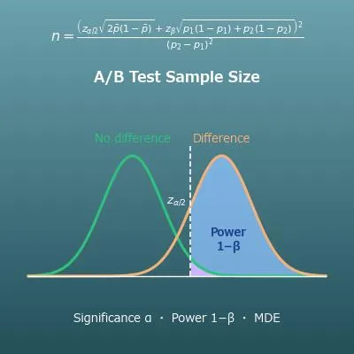
| \(\alpha\) | alpha | The significance level: the probability of calling a difference real when there is none (the probability of a Type I error). 5% (0.05) is the usual choice. Alpha is the first Greek letter, and in statistics it is used for the probability of the "first" kind of error. |
| \(\beta\) | beta | The probability of missing a difference that is really there (the probability of a Type II error). Beta is the second Greek letter, used for the probability of the "second" kind of error. |
| \(1-\beta\) | one minus beta | The power: the probability of finding a difference when there really is one. 80% or 90% is the usual choice. |
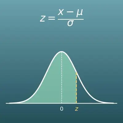
| \(z_{\alpha/2}\) | z sub alpha over two | The z-value for the significance level \(\alpha\) in a two-sided test (the point with \(\alpha/2\) of the standard normal distribution above it). It is 1.9600 at 5%, 2.5758 at 1% and 1.6449 at 10%. A one-sided test uses \(z_{\alpha}\) instead (1.6449 at 5%). |
| \(z_{\beta}\) | z sub beta | The z-value for the power \(1-\beta\) (the point with probability \(1-\beta\) of the standard normal distribution below it). It is 0.8416 at 80% and 1.2816 at 90%. |
| \(z_{1-\beta}\) | z sub one minus beta | In the power formula, the z-value worked back from the sample size. Put it into \(\Phi\) and you get the power. (It is the same thing as \(z_{\beta}\), written from the side of the value you are solving for.) |
| \(\Phi\) | capital phi | The cumulative distribution function of the standard normal distribution. It returns the probability that a z-value is at or below a given value: \(\Phi(1.96) \approx 0.975\) and \(\Phi(0.8416) \approx 0.80\). The capital Greek letter phi is the usual symbol for this function. |
| \(n\) | n | The sample size per group (for each of version A and version B). It stands for number. The total for A and B is \(2n\). |
| \(\sqrt{\ \ }\) | square root | The square root: the positive number that gives the number inside when squared, for example \(\sqrt{30000} \approx 173.205\). It appears when finding the spread (standard deviation) of a CVR. |
| \(V\) | V | Daily visitors (all visits to the page being tested, A and B together). It stands for visits. |
| \(D\) | D | The days needed. It stands for days. |
| \(\lceil\ \rceil\) | ceiling | The symbol for rounding up (the ceiling function). It gives the smallest whole number that is greater than or equal to the number inside (\(\lceil 53.211 \rceil = 54\)). |
Terms
| A/B test | An experiment that splits visitors at random between the current version (A) and a new version (B) over the same period, to see which performs better (for example, has a higher CVR). It is used to check with data, not hunches, whether a change such as a button color, a headline, the way a price is shown or the layout of a landing page really helps. |
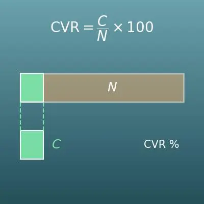
| CVR (conversion rate) | The share of visitors or clicks that end in a goal action (a conversion), such as a purchase or a sign-up. In the formulas on this page, version A's CVR is \(p_1\) and version B's is \(p_2\). |
| MDE (minimum detectable effect) | The smallest lift you want to be able to detect. It is the first value to decide when you plan an A/B test. The smaller it is, the faster the sample size grows (it is inversely proportional to the square of the difference), so choose the smallest lift that would matter to your business. |
| significance level | The probability \(\alpha\) of the mistake you are willing to accept - seeing a chance difference and calling it real when there is no difference. 5% is standard, which allows a false alarm about 1 time in 20. A stricter level (1%) needs a larger sample size. |
| statistical power | The probability \(1-\beta\) of finding a difference when there really is one. 80% is standard, which accepts missing a real lift about 1 time in 5. If a low-power test says "no difference", that is not evidence that there is no difference. |
| Type I error | The mistake of calling a difference real when there is none (a false positive). The probability you allow for it is the significance level \(\alpha\). It is the flip side of a Type II error (a miss): pushing one down tends to push the other up. The most basic way to make both small is a larger sample size. |
| Type II error | The mistake of missing a difference that is really there (a false negative). Its probability is \(\beta\), and \(1-\beta\) is the power. It is the flip side of a Type I error (a false alarm): pushing one down tends to push the other up. The most basic way to make both small is a larger sample size. |
| null hypothesis | The hypothesis "versions A and B have the same CVR" that the test tries to reject. The test asks how unusual the data would be if the null hypothesis were true. If it is unusual enough, the null hypothesis is rejected and the result is "a difference". |
| alternative hypothesis | The hypothesis "versions A and B have different CVRs" that the test tries to show. It is accepted when the null hypothesis (no difference) is rejected. |
| two-sided test | A test that counts both "B is higher" and "B is lower" as a difference. It is used in a normal A/B test, where you do not know which way it will go. It needs a larger sample size than a one-sided test, but it also catches B doing worse. |
| one-sided test | A test that only looks for "B is higher". It needs a smaller sample size than a two-sided test, but it cannot catch B doing worse, so you must choose it before the test starts. (Switching to one-sided after seeing the results is not valid.) |
| two-proportion z-test | A test that checks whether two groups differ in a proportion (such as CVR), using a z-value (the standardized difference) and the standard normal distribution. The formulas on this page find the sample size for this test. The normal approximation works when each group has enough conversions (as a rule of thumb, at least 5 to 10). |
| standard normal distribution | The normal distribution with mean 0 and standard deviation 1 (a symmetric bell shape). A z-value is a point on its horizontal axis, and each z-value matches one probability, as in "the area to the right of 1.96 is 2.5%". |
| cumulative distribution function | A function that returns the probability of getting a given value or less. The one for the standard normal distribution is written \(\Phi\) and appears at the end of the power formula. In Excel it is NORM.S.DIST (with TRUE as the second argument), and in Python it is NormalDist().cdf. |
| standard deviation (spread) | How spread out data is. The spread of a proportion \(p\) is proportional to \(\sqrt{p(1-p)}\). The \(\sqrt{2\bar{p}(1-\bar{p})}\) and \(\sqrt{p_1(1-p_1)+p_2(1-p_2)}\) in the formulas are the spread of the difference between the two groups' CVRs. |
| multiple comparisons | Comparing several B versions or several metrics at the same time. The more comparisons you make, the more likely it is that at least one looks significant by chance, so an adjustment is needed, such as dividing the significance level by the number of comparisons (the Bonferroni correction). |
| peeking (early stopping) | Checking the results again and again before the required sample size is reached and stopping the moment the result looks significant. It makes chance differences easy to catch, so a test meant to have a 5% significance level actually makes wrong calls far more often. The formulas on this page assume that you fix the sample size first and wait until you reach it. |
Good to know before you start
Here is what helps you use the calculation on this page with real understanding, not just by pressing the button.
If you get stuck, going back over these topics is the quickest way forward.
| Percentages (Grade 6) |
|
| Square roots (Grade 8) |
|
| Basic probability (Grade 7 to high school) |
|
| The normal distribution and z-scores (high school statistics) |
|
| The idea of hypothesis testing (AP Statistics or intro college statistics) |
|
| Rounding up (Grade 4) |
|
How to calculate it in Excel
| Baseline CVR p1 (%) | 3 |
| Relative lift r (%) | 10 |
| Target CVR p2 (%) | =B1*(1+B2/100) |
| Baseline CVR p1 (%) | 3 |
| Target CVR p2 (%) | 3.3 |
| Significance level α (%, two-sided) | 5 |
| Power 1−β (%) | 80 |
| z_α/2 | =NORM.S.INV(1-B3/100/2) |
| z_β | =NORM.S.INV(B4/100) |
| Average CVR p̄ | =(B1+B2)/2/100 |
| Sample size per group n (rounded up) | =ROUNDUP((B5*SQRT(2*B7*(1-B7))+B6*SQRT(B1/100*(1-B1/100)+B2/100*(1-B2/100)))^2/((B2-B1)/100)^2,0) |
| Sample size per group n | 53211 |
| Daily visitors V (A + B total) | 2000 |
| Days needed D (rounded up) | =ROUNDUP(2*B1/B2,0) |
| Baseline CVR p1 (%) | 3 |
| Target CVR p2 (%) | 3.3 |
| Significance level α (%, two-sided) | 5 |
| Sample size per group n | 30000 |
| z_α/2 | =NORM.S.INV(1-B3/100/2) |
| Average CVR p̄ | =(B1+B2)/2/100 |
| z_1−β | =(ABS(B2-B1)/100*SQRT(B4)-B5*SQRT(2*B6*(1-B6)))/SQRT(B1/100*(1-B1/100)+B2/100*(1-B2/100)) |
| Power 1−β (%) | =NORM.S.DIST(B7,TRUE)*100 |
The first table shows 3.3 in B3 (a target CVR of 3.3%), the second shows 53211 in B8 (the sample size per group), the third shows 54 in B3 (the days needed) and the fourth shows about 55.71 in B8 (a power of 55.71%).
NORM.S.INV turns a probability into a z-value, and NORM.S.DIST (with TRUE as the second argument) turns a z-value into a probability. For a one-sided test, delete the "/2" from the z_α/2 formula so that it reads =NORM.S.INV(1-B3/100). ROUNDUP(…,0) rounds up.
How to calculate it in Google Sheets
| Baseline CVR p1 (%) | 3 |
| Relative lift r (%) | 10 |
| Target CVR p2 (%) | =B1*(1+B2/100) |
| Baseline CVR p1 (%) | 3 |
| Target CVR p2 (%) | 3.3 |
| Significance level α (%, two-sided) | 5 |
| Power 1−β (%) | 80 |
| z_α/2 | =NORM.S.INV(1-B3/100/2) |
| z_β | =NORM.S.INV(B4/100) |
| Average CVR p̄ | =(B1+B2)/2/100 |
| Sample size per group n (rounded up) | =ROUNDUP((B5*SQRT(2*B7*(1-B7))+B6*SQRT(B1/100*(1-B1/100)+B2/100*(1-B2/100)))^2/((B2-B1)/100)^2,0) |
| Sample size per group n | 53211 |
| Daily visitors V (A + B total) | 2000 |
| Days needed D (rounded up) | =ROUNDUP(2*B1/B2,0) |
| Baseline CVR p1 (%) | 3 |
| Target CVR p2 (%) | 3.3 |
| Significance level α (%, two-sided) | 5 |
| Sample size per group n | 30000 |
| z_α/2 | =NORM.S.INV(1-B3/100/2) |
| Average CVR p̄ | =(B1+B2)/2/100 |
| z_1−β | =(ABS(B2-B1)/100*SQRT(B4)-B5*SQRT(2*B6*(1-B6)))/SQRT(B1/100*(1-B1/100)+B2/100*(1-B2/100)) |
| Power 1−β (%) | =NORM.S.DIST(B7,TRUE)*100 |
How to calculate it in Python
from math import sqrt, ceil
from statistics import NormalDist

base_cvr = 3.0          # baseline CVR (%)
relative_mde = 10.0     # MDE to detect (relative %)
alpha = 0.05            # significance level (two-sided)
power = 0.80            # power
daily_visits = 2000     # daily visitors (A + B total)

p1 = base_cvr / 100
p2 = p1 * (1 + relative_mde / 100)          # target CVR
z_alpha = NormalDist().inv_cdf(1 - alpha / 2)  # for a one-sided test, use 1 - alpha
z_beta = NormalDist().inv_cdf(power)
p_bar = (p1 + p2) / 2

n_exact = (z_alpha * sqrt(2 * p_bar * (1 - p_bar))
           + z_beta * sqrt(p1 * (1 - p1) + p2 * (1 - p2))) ** 2 / (p2 - p1) ** 2
n_per_group = ceil(n_exact)                  # sample size per group (rounded up)
days = ceil(2 * n_per_group / daily_visits)  # days needed

print(f"Target CVR: {p2 * 100:.4g}%")
print(f"Sample size per group: {n_per_group} (total {2 * n_per_group})")
print(f"Days needed: {days}")

# Solving the other way: power with 30,000 visitors per group
n_fixed = 30000
z_power = (abs(p2 - p1) * sqrt(n_fixed) - z_alpha * sqrt(2 * p_bar * (1 - p_bar))) \
          / sqrt(p1 * (1 - p1) + p2 * (1 - p2))
print(f"Power with {n_fixed} per group: {NormalDist().cdf(z_power) * 100:.2f}%")
How to write it in LaTeX and other math languages (copy and paste)
p₂ = p₁ × (1 + r/100)
p_2 = p_1 \left(1 + \dfrac{r}{100}\right)
<math xmlns="http://www.w3.org/1998/Math/MathML" display="block">
  <mrow>
    <msub><mi>p</mi><mn>2</mn></msub>
    <mo>=</mo>
    <msub><mi>p</mi><mn>1</mn></msub>
    <mo>(</mo><mn>1</mn><mo>+</mo><mfrac><mi>r</mi><mn>100</mn></mfrac><mo>)</mo>
  </mrow>
</math>
p_2 = p_1 (1 + r/100)
p1*(1 + r/100)
p2 := p1*(1 + r/100);
p2 = p1*(1 + r/100);
p_2 = p_1 (1 + r/100)
n = (z_α/2 √(2p̄(1 − p̄)) + z_β √(p₁(1 − p₁) + p₂(1 − p₂)))² ÷ (p₂ − p₁)²
n = \dfrac{\left( z_{\alpha/2}\sqrt{2\bar{p}(1-\bar{p})} + z_{\beta}\sqrt{p_1(1-p_1)+p_2(1-p_2)} \right)^2}{(p_2 - p_1)^2}
<math xmlns="http://www.w3.org/1998/Math/MathML" display="block">
<mrow>
<mi>n</mi>
<mo>=</mo>
<mfrac>
<msup>
<mrow>
<mo>(</mo>
<msub><mi>z</mi><mrow><mi>α</mi><mo>/</mo><mn>2</mn></mrow></msub>
<msqrt><mn>2</mn><mover><mi>p</mi><mo>¯</mo></mover><mo>(</mo><mn>1</mn><mo>−</mo><mover><mi>p</mi><mo>¯</mo></mover><mo>)</mo></msqrt>
<mo>+</mo>
<msub><mi>z</mi><mi>β</mi></msub>
<msqrt>
<msub><mi>p</mi><mn>1</mn></msub><mo>(</mo><mn>1</mn><mo>−</mo><msub><mi>p</mi><mn>1</mn></msub><mo>)</mo>
<mo>+</mo>
<msub><mi>p</mi><mn>2</mn></msub><mo>(</mo><mn>1</mn><mo>−</mo><msub><mi>p</mi><mn>2</mn></msub><mo>)</mo>
</msqrt>
<mo>)</mo>
</mrow>
<mn>2</mn>
</msup>
<msup>
<mrow><mo>(</mo><msub><mi>p</mi><mn>2</mn></msub><mo>−</mo><msub><mi>p</mi><mn>1</mn></msub><mo>)</mo></mrow>
<mn>2</mn>
</msup>
</mfrac>
</mrow>
</math>
n = (z_(alpha/2) sqrt(2 bar p (1 - bar p)) + z_beta sqrt(p_1(1 - p_1) + p_2(1 - p_2)))^2 / (p_2 - p_1)^2
Ceiling[(za*Sqrt[2*pbar*(1 - pbar)] + zb*Sqrt[p1*(1 - p1) + p2*(1 - p2)])^2/(p2 - p1)^2]
n := ceil((za*sqrt(2*pbar*(1 - pbar)) + zb*sqrt(p1*(1 - p1) + p2*(1 - p2)))^2/(p2 - p1)^2);
n = ceil((za*sqrt(2*pbar*(1 - pbar)) + zb*sqrt(p1*(1 - p1) + p2*(1 - p2)))^2/(p2 - p1)^2);
n = (z_(α/2) √(2p̄(1 − p̄)) + z_β √(p_1(1 − p_1) + p_2(1 − p_2)))^2/(p_2 − p_1)^2
D = ⌈2n ÷ V⌉
D = \left\lceil \dfrac{2n}{V} \right\rceil
<math xmlns="http://www.w3.org/1998/Math/MathML" display="block">
<mrow>
<mi>D</mi>
<mo>=</mo>
<mo>⌈</mo>
<mfrac><mrow><mn>2</mn><mi>n</mi></mrow><mi>V</mi></mfrac>
<mo>⌉</mo>
</mrow>
</math>
D = |~ (2n)/V ~|
Ceiling[2*n/v]
days := ceil(2*n/V);
D = ceil(2*n/V);
D = ⌈2n/V⌉
1 − β = Φ((|p₂ − p₁|√n − z_α/2 √(2p̄(1 − p̄))) ÷ √(p₁(1 − p₁) + p₂(1 − p₂)))
1 - \beta = \Phi\left( \dfrac{|p_2 - p_1|\sqrt{n} - z_{\alpha/2}\sqrt{2\bar{p}(1-\bar{p})}}{\sqrt{p_1(1-p_1)+p_2(1-p_2)}} \right)
<math xmlns="http://www.w3.org/1998/Math/MathML" display="block">
<mrow>
<mn>1</mn><mo>−</mo><mi>β</mi>
<mo>=</mo>
<mi>Φ</mi>
<mo>(</mo>
<mfrac>
<mrow>
<mo>|</mo><msub><mi>p</mi><mn>2</mn></msub><mo>−</mo><msub><mi>p</mi><mn>1</mn></msub><mo>|</mo>
<msqrt><mi>n</mi></msqrt>
<mo>−</mo>
<msub><mi>z</mi><mrow><mi>α</mi><mo>/</mo><mn>2</mn></mrow></msub>
<msqrt><mn>2</mn><mover><mi>p</mi><mo>¯</mo></mover><mo>(</mo><mn>1</mn><mo>−</mo><mover><mi>p</mi><mo>¯</mo></mover><mo>)</mo></msqrt>
</mrow>
<msqrt>
<msub><mi>p</mi><mn>1</mn></msub><mo>(</mo><mn>1</mn><mo>−</mo><msub><mi>p</mi><mn>1</mn></msub><mo>)</mo>
<mo>+</mo>
<msub><mi>p</mi><mn>2</mn></msub><mo>(</mo><mn>1</mn><mo>−</mo><msub><mi>p</mi><mn>2</mn></msub><mo>)</mo>
</msqrt>
</mfrac>
<mo>)</mo>
</mrow>
</math>
1 - beta = Phi((|p_2 - p_1| sqrt(n) - z_(alpha/2) sqrt(2 bar p (1 - bar p))) / sqrt(p_1(1 - p_1) + p_2(1 - p_2)))
CDF[NormalDistribution[0, 1], (Abs[p2 - p1]*Sqrt[n] - za*Sqrt[2*pbar*(1 - pbar)])/Sqrt[p1*(1 - p1) + p2*(1 - p2)]]
power := Statistics[CDF](Normal(0, 1), (abs(p2 - p1)*sqrt(n) - za*sqrt(2*pbar*(1 - pbar)))/sqrt(p1*(1 - p1) + p2*(1 - p2)));
power = normcdf((abs(p2 - p1)*sqrt(n) - za*sqrt(2*pbar*(1 - pbar)))/sqrt(p1*(1 - p1) + p2*(1 - p2)));
1 − β = Φ((|p_2 − p_1| √n − z_(α/2) √(2p̄(1 − p̄)))/√(p_1(1 − p_1) + p_2(1 − p_2)))
How to have ChatGPT do the calculation
You are an assistant for planning A/B tests. Do the following calculation by actually running Python code, and base your answer only on the numbers from the execution result (do not answer by mental math or guessing).

The current page's CVR (the baseline CVR) is 3%. I want to be able to detect a relative lift of 10% with version B (a CVR of 3.3%).
With a 5% significance level (two-sided test) and 80% power, find each of the following:
1. The target CVR p2 (p2 = p1 × (1 + 10/100))
2. The sample size per group n (the two-proportion z-test formula: n = (z_{α/2}·√(2p̄(1−p̄)) + z_β·√(p1(1−p1)+p2(1−p2)))² ÷ (p2−p1)², with p̄ = (p1+p2)/2, rounded up) and the total sample size for A and B
3. The days needed (rounded up) with 2,000 daily visitors (A and B together)
4. The power if only 30,000 visitors per group are available (1−β = Φ((|p2−p1|·√n − z_{α/2}·√(2p̄(1−p̄))) ÷ √(p1(1−p1)+p2(1−p2))))

Use statistics.NormalDist for the z-values and the cumulative distribution function, and show the formulas you used and the numbers from the execution result.
How to Use
-
1Enter your numbersType the numbers you want to calculate with into the input fields
-
2CalculatePress the "Calculate" button
-
3Check the resultThe result appears on the spot. The same page also explains the idea behind the calculation and the formula
DataChef Features

No technical knowledge required.
Intuitive and user-friendly operation.

Can be used without registering personal information.

Automatic file deletion by clicking "download".

and rapid file conversion.

No attribution required.

No need to contact us for commercial use permission.
Related Features
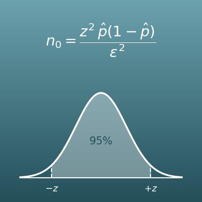
Sample Size Calculator (Surveys and Margin of Error)
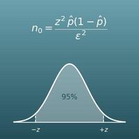
Find how many people a survey needs from the confidence level, margin of error and proportion. Use it when you want to measure one percentage precisely
P-Value Calculator: Z-Score to P-Value and Back
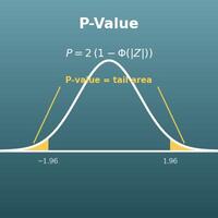
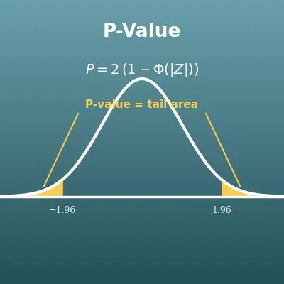
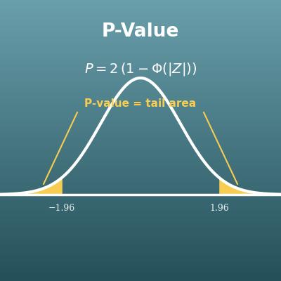
Find the p-value from a z-score and learn when to use a two-sided or one-sided test. It is the other side of the significance level α on this page
Conversion Rate Calculator (CVR, Visitors Needed and Expected Conversions)
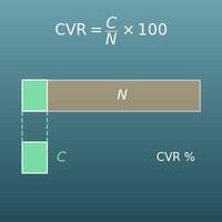
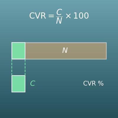
Find visitors, conversions or conversion rate from the other two. Use it to get the baseline CVR for this page
A/B Test Significance Calculator (Conversion Rates, P-Value and Confidence Interval)
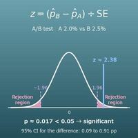
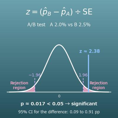
Check whether the difference between A and B is more than chance, with a z-test p-value and confidence interval. Use it after the test ends